
18. Chapter 18: Concluding remarks and perspectives#
Seventeen chapters is a long argument, and it is worth saying plainly what the argument was.
This book has not been a catalogue of methods. A catalogue would have been easier to write and would have dated faster. What it has tried to do instead is to derive a small number of ideas carefully and then follow them until they stop working, because the place where an idea stops working is the place where the next one is invented. Ridge regression stops working when the relationship is not linear, and the sigmoid of Chapter 5 is the smallest possible repair. Logistic regression stops working when the features themselves must be learned, and Chapter 8 inserts a hidden layer. A dense layer stops working when the input is an image, and Chapter 10 replaces full connectivity by a shared local kernel. Maximum likelihood stops working when the normalising constant cannot be computed, and Chapters 14 to 17 are four different ways of proceeding without it. Read in that order the book is not seventeen subjects but one subject seventeen times.
This closing chapter does three things. Section The shape of the argument sets out the shape of the whole and the dependencies between its parts. Section The threads follows the handful of ideas that recur, and argues that they are the part of the material with the longest shelf life. Section A protocol for a new problem turns them round and states them as a working order for attacking a problem that has not been seen before. Sections What this book does not contain and Perspectives then look outward, at what has been left out and at where these methods are being taken in the sciences. Section What to be sceptical about is a list of things to be sceptical about, drawn wherever possible from results in this book that did not come out as expected.
18.1. The shape of the argument#
Figure 18.1 is the book drawn as a graph. It is worth a minute of study, because the interesting thing about it is how few of the arrows are merely chronological.
The two foundational chapters are not preliminaries in the usual sense of material one may skip. Chapter 1 supplies the objects – a data set is a design matrix, a model is a matrix acting on a parameter vector, and fitting is projection onto a column space – and it supplies the one number, the condition number, that reappears in three different roles later. Chapter 2 supplies the discipline: every quantity computed from a finite sample is itself a random variable, with a bias and a variance that the mean squared error of Eq. (2.27) weighs equally. Without the first, the algebra of the later chapters is unreadable; without the second, their numbers are unbelievable.
The five chapters of statistical learning that follow are, deliberately, all the same model seen from different angles. Chapter 3 derives the least-squares estimator three times – as an optimisation problem, as a projection and as a maximum-likelihood estimate – because each derivation generalises differently and the reader needs all three later. Chapter 4 is what happens when the closed form is withdrawn. Chapter 5 changes one function and finds that the loss changes with it, without being chosen. Chapter 6 arrives at a third loss from a geometric principle and finds it belongs to the same family: Ridge regression, logistic regression and the support vector machine are one model with one penalty and three losses, which is the observation Section The primal view: the hinge loss closes on. Chapter 7 is the odd one out and the more valuable for it, because it is the only place in the book where the model is improved not by changing it but by averaging many copies of it, and Eq. (7.16) is the specification that every ensemble in the sciences obeys.
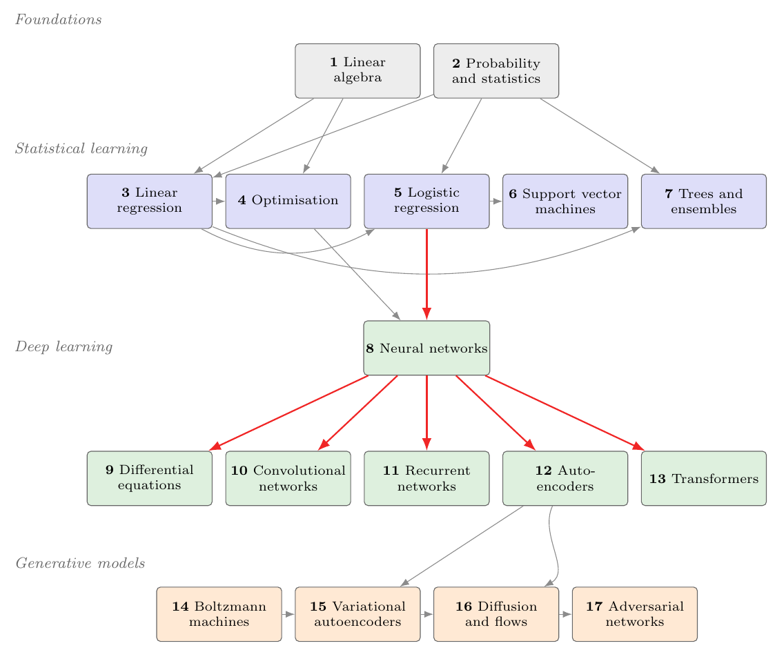
Figure 18.1: The book as a graph. An arrow means that the later chapter uses a result of the earlier one, not merely that it comes after it. The two red paths are the ones the book is built around: logistic regression is a network with no hidden layer, so Chapter 8 begins by inserting one; and Chapters 9 to 13 all use the backpropagation of Section Backpropagation unchanged – Chapters 10 to 13 by changing what structure is imposed on the weight matrix, Chapter 9 by keeping the network and changing the question it is asked. Two links are not drawn because they would cross the whole figure. The linear autoencoder of Chapter 12 rediscovers the singular value decomposition of Chapter 1 – that is Theorem 12.5 – and the Boltzmann machine of Chapter 14 is sampled by the Metropolis algorithm of Section Markov chains and the Metropolis algorithm.
Chapter 8 is the hinge of the book, and the fan of arrows leaving it is the point. Convolutional, recurrent, autoencoding and attention-based networks are not four subjects. They are four answers to a single question – what structure should be imposed on the weight matrix? – and they share, without modification, the four equations of backpropagation derived in Section The four equations of backpropagation. A convolutional layer is a dense layer whose weights are tied and local; a recurrent layer is a dense layer whose weights are tied across time; an autoencoder is a pair of dense stacks with a narrow layer between them; attention is a dense layer whose weights are computed from the data rather than stored. Once that is seen, the differences between the four chapters are differences of consequence, not of kind, and the consequences are what those chapters prove: equivariance under translation (Theorem 10.7) for the first, exponential decay of gradients along the time axis (Theorem 11.1) for the second, an exact identity with principal component analysis (Theorem 12.5) for the third, and equivariance under all permutations (Theorem 13.2) for the fourth.
The last four chapters change the question. Everything before them predicts a target given an input; these model the distribution of the data itself. That change costs one thing and one thing only, and it is worth naming precisely because the whole part is organised around it: a probability model needs a normalising constant, and the normalising constant is a sum or an integral over a space too large to touch. Chapter 14 refuses to compute it and samples instead. Chapter 15 bounds it. Chapter 16 sidesteps it in one direction by learning a score and in the other by restricting to maps whose Jacobian determinant is cheap. Chapter 17 abandons likelihood altogether and trains a classifier in its place. Four chapters, four evasions of the same obstruction; we return to this in Section An intractable normalisation, and four ways round it.
18.2. The threads#
The methods in this book will age at different rates. The ideas that connect them will age more slowly, and this section collects the ones that recurred often enough to be worth carrying away independently of any architecture.
18.2.1. One number governs accuracy, variance and training time#
The condition number \(\kappa_2(\bm{X})=\sigma_0/\sigma_{r-1}\) appeared three times in three different roles, and it is the same number each time.
In Section Vector and matrix norms it decides how much of the input precision survives a linear solve, and the observation that \(\kappa_2(\bm{X}^{T}\bm{X}) =\kappa_2(\bm{X})^{2}\) is why the least-squares routines one should actually call are built on the QR decomposition or the singular value decomposition rather than on the normal equations. In Section Statistical properties of the least-squares estimator the same quantity governs the statistical variance of the fitted parameters, through \(\var(\hat{\bm{\theta}})=\sigma^{2}(\bm{X}^{T}\bm{X})^{-1}\): directions in which the data are uninformative are exactly the directions in which the estimate is uncertain. And in Chapter 4, Eq. (4.27) shows that it sets the number of gradient-descent iterations, because the step size is bounded above by the largest eigenvalue of the Hessian while progress is governed by the smallest.
Three apparently unrelated difficulties – numerical, statistical and computational – are therefore one difficulty. This has a practical consequence that is easy to state and easy to forget: standardising the features and adding a Ridge penalty improve all three at once, and they do so for the same reason. A student who leaves this book remembering only that a badly conditioned design matrix is bad news in three separate ways has taken away something that will outlast every architecture in it.
18.2.2. The loss is derived, not chosen#
The single most useful habit this book has tried to instil is to stop treating the loss function as a design decision. Specify what the target is assumed to be, and the loss follows.
Gaussian noise gives the squared error, Eq. (3.27). Bernoulli observations give the cross entropy, Eq. (5.13); the notebox in Section Deriving least squares from a probability distribution predicted this before Chapter 5 confirmed it. A categorical target gives the multiclass cross entropy, and the softmax that pairs with it is not a convenience but the inverse link of the same model. Non-negative unbounded data suggest a Poisson likelihood and a different loss again. Even the penalties are not free choices: Section A Bayesian reading showed that a flat prior gives ordinary least squares, a Gaussian prior gives Ridge, and a Laplace prior gives the Lasso, so that regularisation is a prior belief and the regularisation parameter is its strength.
The habit pays off most in the last part of the book, where the models are strange. A restricted Boltzmann machine’s loss is the negative log-likelihood of a canonical ensemble, and Theorem 14.2 is nothing but its derivative. A variational autoencoder’s loss is a bound on the same log-likelihood, Theorem 15.1. A diffusion model’s loss looks like a plain squared error, Eq. (16.9), and it is startling to discover that it is one – but it is one only after a variational derivation that begins from a likelihood. Even the adversarial loss of Chapter 17, which appears to break the pattern entirely, turns out by Theorem 17.3 to be minimising a divergence between distributions. In every case the object being minimised was determined by a modelling assumption, and in every case knowing which assumption tells you when the method will fail.
The reverse reading is the useful one
If a loss function is being used whose generating assumption cannot be named, that is a fact about the model, and usually a fact worth discovering early. Squared error on bounded data assumes Gaussian noise on a quantity that cannot be Gaussian, which is why Section Structure recommends a logistic output and the binary cross entropy for pixel intensities. A network trained with a loss nobody can justify is a network whose failures nobody will be able to explain.
18.2.3. Bias, variance, and the two ways to trade them#
Equation (2.52) is the most-used result in the book. It says that expected test error decomposes into a bias term, a variance term and an irreducible noise floor, and that the first two move in opposite directions as model complexity grows.
What matters is that the book showed two structurally different ways to exploit it, and they are worth holding apart. The first is regularisation: keep one model and constrain it. Ridge shrinks each singular direction by \(\sigma_i^{2}/(\sigma_i^{2}+\lambda)\), hardest in exactly those directions in which the data are least informative; the Lasso replaces proportional shrinkage by the soft thresholding of Eq. (3.63) and thereby sets coefficients to zero; dropout, weight decay and early stopping do the same job for networks in Section Regularisation and hyperparameters; and the bottleneck, sparsity, contraction and denoising penalties of Section Regularised autoencoders are four more, which the notebox there argues are the same idea four times.
The second is ensembling: keep the complexity and average away the variance. Equation (7.16), \(\var(\bar{f})=\rho\sigma^{2}+(1-\rho)\sigma^{2}/B\), is the entire specification. It says that averaging \(B\) models kills the second term and leaves the first untouched, so the only way to improve further is to decorrelate the members – which is precisely what random forests do by restricting each split to a random subset of features. It also explains, in one line, why deep ensembles remain one of the most reliable uncertainty estimates available for neural networks [lakshminarayanan2017], and why they are expensive.
Boosting reverses the strategy: instead of averaging strong learners to remove variance, it sums weak ones to remove bias. That gradient boosting turns out to be gradient descent performed in function space is the kind of connection this book has looked for throughout, and it is the reason Chapter 7 sits where it does rather than being relegated to an appendix.
18.2.4. The chain rule is enough#
Chapter 8 opened by admitting that inserting a hidden layer costs every guarantee the previous chapters relied on: no convexity, no closed form, no normal equations, no Karush-Kuhn-Tucker conditions to check the answer against. What was left was gradient descent and the chain rule, and the rest of the book is a demonstration that this is enough.
The four equations of Section The four equations of backpropagation are used, unmodified, by every architecture that follows. The convolutional gradients of Section Backpropagation through a convolutional layer are those equations with the sum restricted by the kernel’s support; backpropagation through time is those equations on an unrolled graph with the gradients from every step summed into shared parameters; attention differentiates like any other composition of matrix products and a softmax. The forward-mode recursions of Chapter 9 are the same calculus run in the other direction, propagating derivatives with respect to the input rather than the parameters, at one extra matrix product per layer per order.
The cost accounting is what makes it practical, and it is worth restating because it is the reason deep learning is possible at all. Backpropagation delivers the gradient with respect to all parameters for about twice the cost of a forward pass, independently of how many parameters there are. Finite differences would need one forward pass per parameter. For a model with \(10^{6}\) weights the difference is between a second and a fortnight, and for a model with \(10^{11}\) weights it is the difference between a research programme and an impossibility. This is not a fact about neural networks; it is reverse-mode automatic differentiation, Section Automatic differentiation, and it applies to any differentiable computation, including the classical simulation codes that readers of this book are likely to have written.
18.2.5. Structure is a prior, and it is the cheapest one available#
The three architecture chapters make the same argument with different symmetries, and it is the argument that most repays generalisation to a new problem.
A dense layer on a colour image of side \(L\) has \(9L^{4}\) weights, which is ten billion for a modest photograph. A convolutional layer has \(K(CF^{2}+1)\), independent of the image size. The saving is bought by two assumptions – locality and stationarity – and Chapter 10 is careful to insist that both are properties of the data and not of the method. For images they hold; for a table of unrelated clinical measurements they do not, and a convolutional layer would be an actively bad choice. Theorem 10.7 turns the informal claim into an exact statement: convolution commutes with translation, so a feature learned in one place is available everywhere. Chapter 13 then makes the complementary choice. Attention is equivariant under all permutations, a far larger group, which is why it assumes almost nothing about the data – and why position must be handed back to it explicitly through the encoding of Proposition 13.5.
The lesson generalises well beyond these two cases, and it is the single most transferable idea in the book for a reader working in the physical sciences. A symmetry of the problem, built into the architecture, is a prior that costs no data to enforce and cannot be violated by the fit. Equivariant graph networks enforce rotations and translations in three dimensions exactly, and the consequence is dramatic: interatomic potentials of the NequIP and MACE families [batzner2022,batatia2022] reach chemical accuracy from training sets some two to three orders of magnitude smaller than non-equivariant architectures require. Data efficiency bought by symmetry is the most reliable free lunch in the subject – and Section What to be sceptical about will note that there are few others [wolpert1997].
18.2.6. One decomposition, read several ways#
Chapter 1 closes by observing that the singular value decomposition separates the part of a problem that carries information from the part that does not, and that the same list of singular values answers five different questions. The rest of the book kept finding a sixth.
The numerical rank of a design matrix, the distance of a feature set from collinearity, the variance retained by a projection, the best low-rank approximation by Eq. (1.124), and the shrinkage applied by Ridge in Section Ridge regression through the singular value decomposition are the five. The sixth is Theorem 12.5: a linear autoencoder trained by gradient descent on reconstruction error recovers the principal subspace, so that the most fashionable architecture of the deep-learning part and the oldest tool of multivariate statistics are, in the linear case, the same object. That theorem is the reason Chapter 12 is worth its length. It gives the exact floor – the Eckart-Young error – against which a nonlinear autoencoder must be measured, and without such a floor the claim that a nonlinearity helped is untestable.
The generalisation is worth stating: whenever a method compresses, ask what it would do if it were linear, and whether the linear answer is available in closed form. If it is, that answer is the baseline, and a method that fails to beat it has not earned its extra parameters.
18.2.7. An intractable normalisation, and four ways round it#
The generative part of this book is organised around a single obstruction. A probability model must integrate to one, and the constant that makes it do so is a sum over a space of size \(2^{M+N}\) for a Boltzmann machine, or an integral over all latent configurations for a latent-variable model. It cannot be computed and it will not go away. What can be done is to find a formulation in which it is not needed, and the four chapters are four such formulations.
Sample instead of computing. Theorem 14.2 shows that the gradient of the log-likelihood is a difference of two expectations, and neither requires the value of \(Z\) – only samples from the distribution it normalises. Metropolis and Gibbs supply those samples using ratios alone, in which \(Z\) cancels. The price is that the samples are correlated and the chain must be run long enough, and Section How biased is CD-\texorpdfstring{\(k\)}{k}? measures exactly what is lost when it is not: contrastive divergence with a single step gives a gradient wrong by \(33\%\) in magnitude, a bias that averaging cannot remove, whose cosine with the true gradient is nevertheless \(0.986\). It is a short vector pointing very nearly the right way, which is why an algorithm that is provably biased trains perfectly well.
Bound it. Theorem 15.1 replaces \(\log p(\bm{x})\) by a quantity that is computable and never larger, with the gap equal to the divergence between the approximate and the true posterior. Raising the bound and improving the posterior approximation are then one act. The price is that the gap is real and unknown; Chapter 15 measures it by importance sampling and finds it is several nats, so the evidence lower bound is not a tight estimate of the log-likelihood and should not be reported as one.
Learn a score, or restrict the map. Chapter 16 makes both moves. A diffusion model never represents a density; it learns \(\nabla_{\bm{x}}\log p\), in which the normalisation has been differentiated away, and Proposition 16.4 identifies the trained noise-prediction network with exactly that object. A normalizing flow takes the opposite route and keeps the density exactly, by restricting to invertible maps whose Jacobian determinant is cheap, Theorem 16.5.
Replace the likelihood by a classifier. Chapter 17 gives up on densities entirely. Proposition 17.1 shows that an optimal discriminator is a density ratio in disguise, and Theorem 17.3 that the generator is then minimising a Jensen-Shannon divergence. The price is that the training problem is a game rather than a minimisation, and games need not converge: the chapter measures a simultaneous iteration diverging exactly as \((1+\gamma^{2})^{t/2}\) on a bilinear problem, and an alternating one circulating forever.
Four evasions, four different prices. A reader who understands the obstruction will be able to place the next generative model to appear – flow matching, consistency models, whatever follows – by asking which of the four routes it takes, and what it therefore has to give up.
18.2.8. Representability is not learnability, and neither is generalisation#
Section The universal approximation theorem spends its length distinguishing three questions that are routinely run together, and the distinction is worth carrying away as a discipline of thought.
Can the model class contain the function? For networks the answer is almost always yes, and Theorem 8.2 makes it quantitative in one dimension: \(N\) rectified units suffice for an error \(L(b-a)/2N\), with the weights written down rather than proved to exist. Will gradient descent find it? Section Representability is not learnability runs the two side by side at matched width and finds that training falls further behind the constructed network as the width grows – a factor of \(5.3\) at \(N=64\) – and that a poor initialisation is a larger handicap than the optimisation itself. And will the result generalise? That is Eq. (2.52), and it is a statement about the model class, the data and the estimator together, which no approximation theorem addresses.
The same three-way distinction organises the honest reading of the rest of the book. Theorem 8.6 shows a function a deep network represents exactly and a shallow one provably cannot approximate – a statement about representability, proved in half a page. Theorem 11.1 shows that a recurrent network’s gradients decay exponentially with lag – a statement about learnability, which is why the long-memory tasks of Chapter 11 fail even when the architecture could express the answer. And the experiment of Section Does it actually help? An experiment shows a convolutional network with \(2.5\) times fewer parameters beating a dense one by seventeen points of accuracy on shifted digits while being indistinguishable from it on centred ones – a statement about generalisation, and about the fact that an architectural advantage exists only when the data have the structure the architecture assumes.
18.3. A protocol for a new problem#
The threads of Section The threads are not only retrospective. They compose into a working order for attacking a problem that has not been seen before, and it is worth writing that order out, because the most common way to waste six months is to begin at step six.
1. Say what the target is. Not what model you intend to use – what the quantity being predicted actually is. Continuous and unbounded, bounded to an interval, non-negative, a count, a category, an ordered category, a direction, a distribution. This determines the output activation and, by Section The loss is derived, not chosen, the loss; and the question is worth asking before any code is written because it is frequently the question that reveals the problem has been posed wrongly. If no distributional assumption can be named, the loss cannot be justified, and every later disagreement about which model is better will be an argument about an arbitrary choice.
2. Look at the design matrix before the model. Compute the singular values. The condition number tells you three things at once by Section One number governs accuracy, variance and training time – how much precision a solve will lose, how uncertain the fitted parameters will be, and how slowly gradient descent will converge – and the decay of the spectrum tells you the effective dimension of the problem, which is usually far smaller than the number of columns. Standardise, and know why you are standardising. This step costs minutes and routinely changes what is attempted next.
3. Fix the evaluation before fitting anything. Decide the split, and decide it according to the structure of the data rather than at random: temporally ordered data need a temporal split, grouped data need a grouped split, and spatial data need a spatial one, because the alternative is the leakage of Section What to be sceptical about and it will flatter every result that follows. Decide the metric, and decide it from the decision the model is meant to support – Section Measuring the quality of a classifier on why accuracy is close to meaningless under class imbalance is the relevant caution. Decide, in advance, what difference would count as a real difference; and since almost every method in this book has a seed-to-seed spread, plan to run several seeds and report the spread rather than the best.
4. Fit the linear model. Ordinary least squares, Ridge, logistic regression, whichever the target dictates. It takes an afternoon, it has a closed form or a convex objective, its uncertainty is available analytically, and it is interpretable. It is also, surprisingly often, competitive. Whatever comes later must beat this number, and a great deal of published work would look different if this step were mandatory.
5. Try the ensemble of trees. Gradient boosting on tabular data remains extremely hard to beat, it needs no feature scaling, it is invariant under monotone transformations of the inputs, and it will tell you which features matter. If the data are a table of heterogeneous measurements, this may well be the end of the exercise; the architectural arguments of Chapters 10 to 13 assume structure that a table does not have, and Section Why not simply use a dense layer? is explicit that a convolutional layer applied to unrelated clinical measurements is an actively bad choice.
6. Only now ask what structure the data have. A network earns its place when there is structure for an architecture to exploit. Locality and stationarity along one or more axes point at a convolution; an ordering that must be respected and a state that must be carried points at a recurrence; a set with no natural order, or long-range interactions between elements, points at attention; a graph points at message passing; a known symmetry group points at an equivariant architecture, which by Section Structure is a prior, and it is the cheapest one available is the most data-efficient constraint available. If none of these apply, the honest answer is that a network is unlikely to help, and step five was the answer.
7. Establish the floor before claiming the ceiling. Whatever the nonlinear model is, find the linear version of it and fit that first. For an autoencoder the linear version is principal component analysis and its error is the Eckart-Young value, known exactly by Theorem 12.5. For a sequence model it is an autoregressive fit. For a physics surrogate it is the existing numerical scheme, and Section When is this worth doing? is a cautionary example of what happens when that comparison is actually run: finite differences beat the neural solver by orders of magnitude in time at comparable accuracy. A nonlinear model that does not clear its own linear floor has not earned its parameters.
8. Verify the gradient, then the model. Before trusting an implementation, check it against something that cannot be wrong: finite differences for a hand-written gradient, an analytic special case, a small enough instance to enumerate exactly, or an independent implementation in a second framework. This book does all four at various points, and it does so because a wrong gradient does not announce itself – the network still trains, just to the wrong place. The cost is an hour; the alternative is discovering the error after the results are written up, or not at all.
9. Report what happened. Including the seeds, including the spread, including the configurations that did not work, and including the baseline that was not beaten. The negative result of Section Does it actually help? An experiment took as long to produce as a positive one would have, and it is more informative than most positive results, because it says precisely when the method helps and when it does not.
The order matters more than the list
Every item above is standard advice. What is not standard is doing them in this order, and the reason to insist on it is that steps one to five are cheap and answer the question “is there signal, and how much?”, while steps six onwards are expensive and answer only “can I extract a little more of it?”. A project that reaches step six without a number from step four has no way of knowing whether anything it does afterwards is an improvement.
18.4. What this book does not contain#
A book has to stop somewhere, and it is more useful to say where than to pretend the boundary is a natural one. Five omissions are large enough that a reader should know they are omissions rather than gaps in the subject.
Reinforcement learning.
Every method in this book learns from a fixed data set. Reinforcement learning learns from interaction: an agent takes actions, receives rewards, and must trade exploration against exploitation without ever being told what the correct action was. The mathematics is different enough to need its own treatment – Markov decision processes, the Bellman equations, temporal-difference learning, policy gradients – and the standard reference remains Sutton and Barto [sutton2018]. What connects it to this book is that modern reinforcement learning is deep learning with a different loss: the value function or the policy is a network trained by the backpropagation of Chapter 8, and the innovations that made it work at scale, from the replay buffer and target network of deep \(Q\)-learning [mnih2015] to the clipped surrogate objective of proximal policy optimisation [schulman2017], are all devices for making a non-stationary regression problem behave like a stationary one. Section Reinforcement learning and agentic systems returns to what it is being used for.
Graph neural networks.
Chapters 10 and 13 cover two extremes of structural assumption: a grid with translation symmetry, and a set with full permutation symmetry. Most scientific data lie between them. A molecule, a crystal, a mesh, an interaction network and a particle-physics event are all graphs, and the architecture that respects a graph’s structure is message passing, in which each node updates its state from its neighbours [gilmer2017]. Everything in Section Structure is a prior, and it is the cheapest one available applies: a graph network is a dense layer whose weights are shared across edges, it is equivariant to relabelling of the nodes, and adding equivariance under rotations and translations of the embedding space [fuchs2020,batzner2022,batatia2022] is what makes it useful for physics. A reader who has understood Chapter 10 has most of what is needed.
Uncertainty quantification.
This book computes point predictions and reports test errors. It does not say what a prediction’s uncertainty is, and for scientific use that is often the number that matters. Three practical routes exist. Deep ensembles [lakshminarayanan2017] are the ensembling of Section Bias, variance, and the two ways to trade them applied to networks and remain a strong default. Bayesian deep learning places a posterior over weights and approximates it, usually variationally, which is Chapter 15’s machinery pointed at the parameters rather than at a latent code. Conformal prediction [angelopoulos2023] is different in kind and deserves to be far better known in the sciences: it wraps any predictor whatever in a procedure that produces intervals with a finite-sample coverage guarantee, assuming only exchangeability, and it is the only one of the three that promises anything provable.
Scale.
Everything in this book runs on a laptop, deliberately, so that the reader can reproduce every number. Nothing here therefore prepares one for the regime in which the current large models operate, where the empirical scaling laws [kaplan2020] relating loss to parameters, data and compute are the main design tool, and where the engineering – distributed training, mixed precision, data pipelines, checkpointing – is a large part of the work. The mathematics does not change; the constants do, and the constants decide what is possible.
Everything after the model. Data collection, provenance, versioning, monitoring for drift, and the long maintenance life of a deployed model are absent from this book and are most of the effort in practice. The observation that machine-learning systems accrue technical debt faster than ordinary software is a decade old and has not stopped being true.
18.5. Perspectives#
The rest of this chapter looks outward. What follows is not a survey – the field moves too quickly for a survey in a book to be anything but an embarrassment within two years – but an attempt to say, discipline by discipline, which of the methods derived here are being used, for what, and what is still missing. The references are entry points rather than a bibliography.
18.5.1. Physics#
The application closest to this book’s own machinery is the use of a neural network as a variational ansatz for a quantum many-body wave function. The idea is due to Carleo and Troyer [carleo2017]: represent the amplitude \(\Psi(\bm{s})\) of a spin configuration by a restricted Boltzmann machine, and minimise the energy by the stochastic gradient methods of Chapter 4, sampling configurations by exactly the Metropolis algorithm of Section Markov chains and the Metropolis algorithm. Every ingredient is in this book. The extension to continuous space and to fermions requires an antisymmetric ansatz, and FermiNet [pfau2020] and PauliNet [hermann2020] supply one by embedding determinants in a network; both reach chemical accuracy on small molecules from first principles, with no basis set. The obstruction is the one Chapter 14 identified – the normalisation is unavailable, so everything is done with ratios and samples – and the sign problem in its usual form is not solved but re-expressed.
In high-energy physics the pattern is different: the data are abundant and the task is classification. Deep networks for the identification of exotic particles [baldi2014] were among the first demonstrations that a network could outperform hand-engineered high-level features, and jet tagging is now routinely done with graph networks over particle constituents. The generative part of this book is what is being used for the reverse problem, fast simulation: a calorimeter shower takes seconds to simulate exactly and microseconds to generate with a trained model, and both adversarial and diffusion-based generators are in production use. The scientific question that then arises is the one Chapter 17 warns about – a generator that reproduces every summary statistic examined may still not reproduce the one that has not been examined – which is why validation of such surrogates is an active field in its own right rather than a formality.
In condensed matter, the classification of phases directly from configurations by a convolutional network [carrasquilla2017] showed that an order parameter need not be known in advance to be detected, and machine-learned interatomic potentials have changed what molecular dynamics can reach [batzner2022,batatia2022,merchant2023]. In astrophysics and cosmology the generative methods of Chapters 15 to 16 are used for field-level inference, for denoising gravitational-wave strain, and increasingly as learned priors inside otherwise classical inference pipelines – which is, in the language of Section The loss is derived, not chosen, an admission that the prior was the part nobody could write down.
18.5.2. Chemistry and materials science#
Chemistry is where the graph representation of Section What this book does not contain is not a modelling choice but the natural encoding of the object, and it is the discipline in which machine learning has so far changed practice most.
Property prediction from molecular graphs by message passing [gilmer2017] and its equivariant descendants [schutt2018,batzner2022,batatia2022] now supplies energies and forces at a small fraction of the cost of the electronic structure calculation they are trained on, which moves molecular dynamics from picoseconds to microseconds at density-functional accuracy. The consequence at scale is a discovery pipeline: the systematic search reported by Merchant and co-workers [merchant2023] added of the order of \(10^{5}\) predicted stable crystals to a field that had accumulated a few tens of thousands over its history. The caveat is the one of Section Limitations, and a top-down view: such models interpolate within the chemistry they were trained on and extrapolate unpredictably outside it, and a stability prediction is not a synthesis.
Generation is the other half. A molecule is a discrete object, so the continuous generative models of Chapters 15 to 16 must be adapted rather than applied, and the practical answer has been to diffuse in a continuous latent space or over atomic coordinates directly. Flow matching [lipman2023] has become a favoured alternative because it trains by regression on a velocity field, avoiding both the adversarial game of Chapter 17 and the long sampling chains of Chapter 16. For quantum chemistry proper, the physics-informed formulation of Chapter 9 is being applied to the electronic Schr”odinger equation, and the caution recorded there applies with force: a rectified network has \(f''\equiv0\) and will report a residual of zero while failing to solve a second-order equation at all.
18.5.3. Mathematics: operators, inverse problems and guarantees#
Chapter 9 solves a differential equation by fitting one solution. Operator learning changes the object of the fit: instead of approximating \(u\), approximate the map from the coefficient function, or the initial condition, to the solution. DeepONet [lu2021] builds this from a branch network acting on the input function and a trunk network acting on the query point; Fourier neural operators [li2021fno] parameterise the kernel in Fourier space and are therefore resolution-independent, so a model trained on a coarse grid evaluates on a fine one. Once trained, a new instance costs a forward pass rather than a solve, which is what makes these methods attractive for many-query problems – optimisation, control, uncertainty propagation – and irrelevant for a single high-accuracy solve, exactly as Section When is this worth doing? argued for physics-informed networks [raissi2019,karniadakis2021].
Inverse problems are the natural home of the generative part of this book. The classical difficulty is that a regularising prior has to be chosen by hand, and the modern answer is to learn it: a diffusion model trained on plausible solutions supplies a score, and the score can be used inside a sampler that also respects the measurement. What is obtained is not a single reconstruction but a sample from an approximate posterior, which is the right object – and it inherits, without dilution, the warning of Section An intractable normalisation, and four ways round it that “approximate” is doing real work in that sentence.
Two further directions are worth naming. Symbolic regression aims to recover an equation rather than a black box, and the combination of a graph network with a symbolic fit to its learned messages [cranmer2020] has recovered known force laws from simulation data, which is the most direct attack there is on interpretability. And the guarantee side of the subject is finally maturing: conformal prediction [angelopoulos2023] converts any predictor into one with finite-sample coverage, which is the sort of statement the sciences ought to be demanding as a matter of course.
18.5.4. Earth, ocean and climate science#
Numerical weather prediction is the clearest case in any science of a data-driven model displacing a physical one on the physical model’s own terms. GraphCast [lam2023] is a graph network over a multi-mesh discretisation of the globe, trained on decades of reanalysis, and it produces a ten-day forecast in about a minute on a single accelerator, outperforming the operational deterministic system on the large majority of verified variables. FourCastNet [pathak2022] reaches comparable skill from a Fourier neural operator. Neither model knows any physics. Both are trained by the loss of Section The loss is derived, not chosen on the trajectory of a system whose equations we have known for a century.
It is worth being precise about what this does and does not show. It shows that where a very large, homogeneous, quality-controlled record exists, and where the target is a short-horizon forecast, learning the propagator can beat integrating the equations at a fraction of the cost. It does not show that the equations are dispensable: the training data are themselves the output of a physical assimilation system, the models inherit its biases, and their behaviour under a climate they have not seen is exactly the extrapolation regime Section Limitations, and a top-down view warns about. The interesting research is consequently in hybrid schemes, where a learned component sits inside a physically constrained solver and is responsible only for what the solver parameterises.
In seismology the convolutional and recurrent architectures of Chapters 10 and 11 have made detection of small events routine, lowering magnitude-of-completeness thresholds enough to change what catalogues contain. In remote sensing the multi-modal transformer is becoming the default for fusing spectral bands, radar and time series, and in subsurface imaging generative models supply the prior for reservoir characterisation – again, a learned prior standing in for one nobody could write down.
18.5.5. Bioscience and medicine#
The prediction of protein structure from sequence is the field’s most cited success, and it is instructive because of how many threads of this book it combines. AlphaFold2 [jumper2021] is attention (Chapter 13) over a representation of evolutionary couplings, followed by a structure module equivariant under rigid motions (Section Structure is a prior, and it is the cheapest one available), trained end to end by backpropagation (Chapter 8) on a curated database. Language-model approaches [lin2023] dispense with the alignment and predict structure from a single sequence, trading a little accuracy for a large speed-up; later systems extend the same architecture to complexes and ligands [abramson2024]. Design is the inverse problem, and it is now done with the generative machinery of Chapter 16: RFdiffusion and its relatives [watson2023] sample backbones conditioned on a functional site, and the designs are synthesised and tested, which is the only validation that counts.
Elsewhere in the life sciences the pattern is more familiar. Variational autoencoders are the standard tool for single-cell transcriptomics, where the latent space of Chapter 15 is used as a coordinate for cell type and developmental trajectory – and where the notebox of Section Reconstruction, projection and representation is worth rereading, since a low reconstruction error is evidence that information survived the bottleneck and not that it survived in an interpretable form. Medical imaging uses convolutional and, more recently, diffusion-based models for segmentation and anomaly detection; the distinguishing feature of the domain is that the cost of a false negative is not symmetric with the cost of a false positive, so the confusion-matrix vocabulary of Section Measuring the quality of a classifier is not optional and accuracy is close to meaningless.
18.5.6. Reinforcement learning and agentic systems#
Reinforcement learning is the part of machine learning whose scientific applications look least like the rest of this book, because the model is not fitted to a data set but improved against an environment.
The demonstration most likely to convince a physicist is the magnetic control of a tokamak plasma by a learned policy [degrave2022]: a network trained entirely in simulation, deployed on a real device, holding a variety of plasma configurations that would each traditionally have required a separately designed controller. The pattern – train in a simulator that is good enough, transfer to the apparatus, keep a classical safety layer underneath – is the template for most of what is currently promising, and it puts the burden squarely on the simulator. Related work is under way on pulse sequences for quantum control and error correction, on adaptive experimental design, where the agent chooses the next measurement rather than the next action, and on the exploration of chemical space under a property reward.
The methodological caution is severe and should be stated. Reinforcement learning has the weakest reproducibility record of anything in this book: results are famously sensitive to random seeds, implementation details and reward shaping, and the difference between two published algorithms is often smaller than the spread across seeds of either. A reader coming from the discipline this book has tried to instil – report the spread, quote the seed, publish the program – will find that discipline is needed there more than anywhere else.
The newest development, and the one hardest to assess soberly, is the use of language-model-based agents to run parts of the scientific process itself: proposing hypotheses, writing and executing analysis code, calling simulators, reading literature, and iterating on the result. Systems of this kind now perform real work in literature synthesis and code generation, and the honest summary is that they are useful where the output can be checked cheaply and unreliable where it cannot. That is not a temporary state of affairs to be waited out; it is a statement about verification, and it means the useful question is not how capable such a system is but how the correctness of its output is established. A generated proof can be checked, a generated program can be run against tests, a generated experimental protocol can be executed. A generated literature summary can be checked only by reading the literature.
18.5.7. Foundation models and transfer#
The final trend is the one that most changes how a scientist should approach a new problem. A large model pre-trained on a general corpus – protein sequences, molecular structures, the atmospheric record, sky surveys – can be adapted to a specific task with a small labelled set, because the representation it has already learned does most of the work. The empirical regularity underlying this is the scaling behaviour of [kaplan2020], and the practical consequence is that the first question about a new problem is no longer “what architecture?” but “what pre-trained representation exists, and how little data do I need to adapt it?”.
For a scientific reader this cuts both ways. It puts capable models within reach of groups that could never train one, which is a genuine democratisation. It also introduces a dependency on artefacts whose training data, biases and failure modes are frequently undocumented, and which cannot be interrogated with the tools of this book because their weights or their corpora, or both, are not available. Reproducibility in the sense this book has insisted on – run the program, get the number – is not currently achievable for results that rest on such a model, and pretending otherwise does the field no service.
18.6. What to be sceptical about#
This book has reported, deliberately, several results that did not come out as hoped, on the principle that a method’s failures are more informative than its successes. Collected here, they make a serviceable checklist.
A baseline you did not try honestly is not a baseline. Section Does it actually help? An experiment compares a convolutional network with a dense one on centred handwritten digits at matched parameter count and finds \(0.9656\) against \(0.9670\) – a difference far smaller than the spread across seeds of either. The convolutional network is not better. It becomes better, by seventeen points, only when the digits are placed at random offsets, because only then do the data have the structure the architecture assumes. A great many published comparisons would not survive being run this way.
Likelihood is not sample quality. Section Verifying exactness trains a normalizing flow that reports \(5.46\) nats while producing useless samples, by contracting the data into a region where the prior is nearly flat and harvesting the Jacobian term. The likelihood of a continuous density is unbounded above, and a sufficiently flexible model will find that out. Any single scalar score can be gamed by a model with enough freedom, and the remedy is not a better score but more than one of them, including one that looks at the samples.
An existence proof is not an algorithm. Section Representability is not learnability measures the gap between the network Theorem 8.2 constructs and the network Adam finds at the same width, and the gap grows with width. Universal approximation removes representability as an excuse and leaves optimisation and generalisation, which are the hard parts.
An architecture supplies a path; the initialisation decides whether training starts near it. Section Why it works, and by how much measures an LSTM at \(\bm{b}_f=0\) transmitting \(3.9\times10^{-18}\) of the gradient across fifty-nine steps, against \(1.7\times10^{-18}\) for the vanilla recurrent network it was designed to improve on. The ten to fifteen orders of magnitude usually attributed to the architecture come from biasing the forget gate open. The general form of this error – crediting a structural change with a benefit that came from an initialisation, a schedule or a normalisation shipped alongside it – is extremely common.
A biased estimator can be perfectly useful, and a correct one useless. Section How biased is CD-\texorpdfstring{\(k\)}{k}? finds contrastive divergence wrong by \(33\%\) in magnitude with a cosine of \(0.986\) against the true gradient. It trains well because direction is what gradient descent consumes. Conversely, the flow above is exactly correct about its likelihood and worthless as a generative model. Ask what property of an estimate the algorithm actually uses.
Games are not minimisations. Chapter 17 measures a simultaneous gradient iteration diverging as \((1+\gamma^{2})^{t/2}\) on a bilinear game, and an alternating one circulating forever. Loss curves that oscillate are not a sign of a bad learning rate but the expected behaviour of the dynamics, and “the loss went down” is not evidence of progress in an adversarial setting.
Networks extrapolate unpredictably, and say nothing when they do. This is Section Limitations, and a top-down view, and it is the failure mode that matters most in the sciences, because the interesting regime is so often outside the training distribution. A network gives no signal that it has left the region it was fitted in. This is the strongest practical argument for the uncertainty methods of Section What this book does not contain and for the symmetry constraints of Section Structure is a prior, and it is the cheapest one available, which continue to hold where the data run out.
The most common error is not in the model. It is leakage: a preprocessing step fitted on all the data, a temporal split performed at random, a duplicated record spanning the train-test boundary, a hyperparameter chosen on the test set. A survey across seventeen fields [kapoor2023] found errors of this family affecting hundreds of papers, and their effect is always in the same direction. The rule that prevents all of them is the one stated in Chapter 2 and repeated throughout: anything learned from the data must be learned from the training data only.
And there is no free lunch. Averaged over all problems, no algorithm beats any other [wolpert1997]. Every gain in this book was bought by an assumption – linearity, smoothness, locality, stationarity, a symmetry group, a noise model, a prior – and the method works exactly to the extent that its assumption holds for the data at hand. Choosing a method is choosing an assumption, and it is worth being able to say aloud which one.
18.7. A last word#
The most durable thing this book has to offer is not a method but a habit, and it is worth stating explicitly because it is the habit the field most often lacks.
Every number quoted in these seventeen chapters was produced by a program that accompanies the text, and the programs are collected so that the reader can run them and get the same number. Where a claim could be checked against an exact result, it was: the gradient identity of Chapter 14 against finite differences to \(10^{-8}\), the forward posterior of Chapter 16 against quadrature to six decimals, the optimal discriminator of Chapter 17 to \(3\times10^{-9}\), the linear autoencoder against the singular value decomposition, three independent implementations of every architecture against one another to the precision of double arithmetic. Where the check failed, or where the result was less flattering than expected, that is what appears in the text. This is not pedantry. A field in which a wrong gradient trains almost as well as a right one, in which a model can score well on the metric it is graded by while being useless, and in which the difference between two methods is routinely smaller than the difference between two random seeds, is a field that has to verify rather than believe.
The methods will change. Some of the architectures treated here at length will be of historical interest within a decade, and something not yet published will be in every chapter of the next edition. What will not change is that the loss follows from the model, that the condition number governs three things at once, that structure is a prior worth more than data, that a normalisation which cannot be computed must be evaded rather than ignored, and that a result nobody can reproduce is not a result. Those are the parts worth carrying forward, and they are, not coincidentally, the parts this book has tried hardest to prove rather than assert.
The rest is your problem now, and it is a good time to have it.