
6. Chapter 6: Support Vector Machines#
Logistic regression, in Chapter 5, placed a decision boundary by maximising a likelihood. Support vector machines place one by a different principle: among all boundaries that separate the classes, choose the one that stands as far as possible from the data. This is the maximum margin idea, and it leads to a strikingly different mathematical apparatus – constrained optimisation, Lagrange duality, and the kernel trick that lets a linear method draw non-linear boundaries at almost no extra cost.
The chapter is also where a promise made in Chapter 4 comes due. There we developed unconstrained methods, gradient descent and its descendants. The SVM problem is constrained, and no amount of gradient descent will respect an inequality. We shall therefore derive the dual problem, see that it is a quadratic program, and – rather than reach for a library – construct a solver for it from scratch. The algorithm we build, sequential minimal optimisation, is the one that made support vector machines practical, and it is simple enough to derive in full.
6.1. Hyperplanes and the margin#
Consider two classes of points in a plane. A linear classifier splits the feature space into two half-spaces by placing a hyperplane between them; all points on one side are assigned to one class and all points on the other side to the other. The difficulty, immediately apparent from any picture of separable data, is that there are infinitely many such hyperplanes. Which should we choose?
The support vector machine answers: the one with the maximum margin, the largest distance to the nearest data points of either class. Maximising the margin provides a reinforcement, so that future data points can be classified with more confidence: a boundary that passes close to a training point will misclassify a new point drawn slightly to the other side of it, while a boundary in the middle of a wide corridor has room to spare.
Figure 6.1 shows the solution for two well-separated classes. The solid line is the decision boundary, the dashed lines are the margin hyperplanes \(\bm{w}^{T}\bm{x}+b=\pm1\), and the circled points are those with \(\lambda_i>0\). Two features are worth noticing in advance of the derivation. The circled points lie exactly on the dashed lines, which is the content of the complementary slackness condition (6.19); and there are only three of them out of sixty, so fifty-seven of the observations could be deleted without moving the boundary at all.
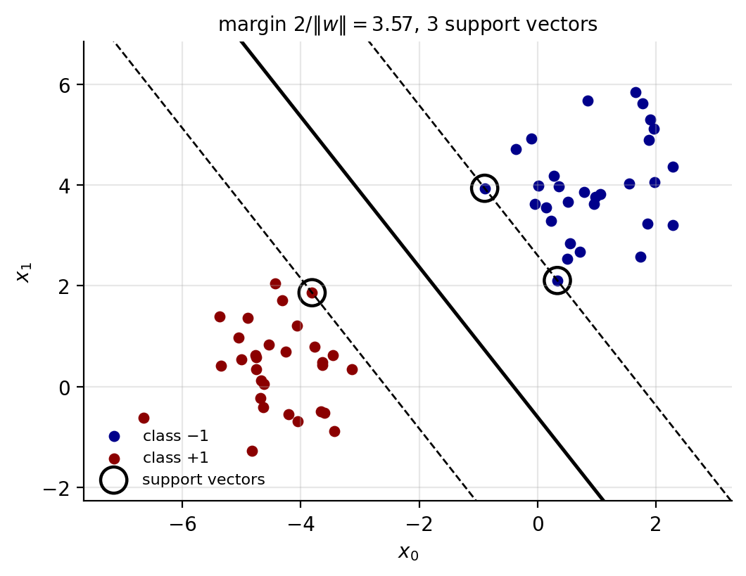
Figure 6.1: The maximum-margin hyperplane for two separable classes. Dashed lines are the margin hyperplanes \(\bm{w}^{T}\bm{x}+b=\pm1\), separated by \(2/\|\bm{w}\|\); circled points are the support vectors, the only observations entering Eq. (6.16).
The geometry. Following the conventions of Chapter 1, define the function
whose zero set is the hyperplane \(L\) separating the classes. Any two points \(\bm{x}_1\) and \(\bm{x}_2\) lying on \(L\) satisfy \(\bm{w}^{T}(\bm{x}_1-\bm{x}_2)=0\), so \(\bm{w}\) is orthogonal to every direction within the hyperplane: \(\bm{w}\) is the normal vector.
The signed distance from an arbitrary point \(\bm{x}\) to \(L\) follows. Writing \(\bm{x}=\bm{x}_0+\delta\,\bm{w}/\|\bm{w}\|\) with \(\bm{x}_0\) on \(L\), so that \(\delta\) is the distance measured along the normal, and applying Eq. (6.1),
The sign tells us which side of the boundary the point lies on and the magnitude how far away it is. Throughout this chapter we label the classes \(y_i\in\{-1,+1\}\) rather than \(\{0,1\}\), which is the convention that makes the algebra of margins clean: the product \(y_i f(\bm{x}_i)\) is then positive exactly when the point is correctly classified.
6.2. A first attempt, and why it fails#
Before constructing the margin, it is instructive to try the obvious thing. Define a cost function running over the set \(M\) of currently misclassified points,
where a point is counted as misclassified when \(y_i=+1\) but \(\bm{w}^{T}\bm{x}_i+b<0\), or the reverse. Each term in the sum is positive for a misclassified point, so the cost measures the total extent of the errors. Differentiating,
and we may descend with any method of Chapter 4,
with \(\gamma\) the familiar learning rate. This is the perceptron algorithm, and the framework is that of logistic regression in Chapter 5.
It works, after a fashion, and its defects are instructive. If the data are separable it converges to some separating hyperplane, but which one depends on the initialisation and the order of the updates – the algorithm stops as soon as \(M\) is empty, wherever that happens to be, so it will happily return a boundary grazing the data. When the gap between the classes is small it may need very many iterations. And if the data are not separable the set \(M\) never empties and the iteration does not converge at all.
The maximum-margin formulation fixes all three defects at once: the solution is unique, it is characterised by a clean optimisation problem, and the soft version of Section The soft margin handles non-separable data gracefully.
6.3. The maximum-margin problem#
We seek a margin \(M\), with \(\bm{w}\) normalised so that \(\|\bm{w}\|=1\), subject to
which says that every point lies at signed distance at least \(M\) from the boundary, on the correct side. Dropping the normalisation and using Eq. (6.2), the condition reads
Now comes the step that makes the problem tractable. Equation (6.1) is unchanged if \(\bm{w}\) and \(b\) are both multiplied by a positive constant, so the pair \((\bm{w},b)\) is determined only up to scale and we are free to fix that scale however we like. Choosing \(\|\bm{w}\|=1/M\) turns the right-hand side of Eq. (6.7) into unity, and the problem becomes
The margin is now the inverse of the norm: since \(M=1/\|\bm{w}\|\) and the corridor extends by \(M\) on each side, the total width between the two classes is \(2/\|\bm{w}\|\). Maximising the margin is therefore minimising the norm, and the factor \(\tfrac12\) is inserted purely so that the derivative comes out clean.
Equation (6.8) is a convex problem – a quadratic objective with linear inequality constraints – so by Section Convexity it has a unique global minimum. But the methods of Chapter 4 cannot be applied directly, because they know nothing of constraints. We need Lagrange multipliers.
6.4. A reminder on Lagrange multipliers#
Consider a function \(f(x,y,z)\) of three independent variables. For \(f\) to be extremal we require \(df=0\), and since
a necessary and sufficient condition is that all three partial derivatives vanish.
In many problems, however, the variables are subject to constraints and are no longer independent. In principle one could use each constraint to eliminate a variable and proceed with a smaller independent set. Lagrange’s method is the alternative when elimination is inconvenient or destroys the symmetry of the problem.
Suppose the variables satisfy a constraint
We may no longer set the three partial derivatives of \(f\) separately to zero, because only two of the variables are independent: if \(x\) and \(y\) are chosen freely then \(dz\) is determined. But since \(d\phi=0\), we may add \(\lambda\,d\phi\) to \(df\) for any multiplier \(\lambda\) without changing anything,
We now choose \(\lambda\) so that the coefficient of the dependent differential \(dz\) vanishes. The remaining two differentials are independent and arbitrary, so their coefficients must vanish too, and we obtain the three symmetric conditions
together with the constraint \(\phi=0\) itself – four equations for the four unknowns \(x,y,z,\lambda\). Equivalently, we form the Lagrangian \(\mathcal{L}=f+\lambda\phi\) and treat all variables, the multiplier included, as independent.
For inequality constraints of the form \(\phi\ge0\) the situation is richer, and the conditions that replace Eq. (6.12) are the Karush-Kuhn-Tucker conditions, which we shall meet in Eq. (6.19). The essential addition is that a multiplier belonging to an inequality must be non-negative, and that it vanishes whenever its constraint is satisfied strictly – a constraint that is not binding exerts no force.
6.5. The dual problem#
We attach a multiplier \(\lambda_i\ge0\) to each of the \(n\) inequality constraints of Eq. (6.8) and form the Lagrangian
The sign is chosen so that violating a constraint – making the bracket negative – increases \(\mathcal{L}\), which is what a penalty should do.
Differentiating with respect to the primal variables, using Eqs. (1.25) and (1.28) from Section Four worked examples,
The second is worth pausing over. It says
that the optimal normal vector is a linear combination of the training points, with the labels supplying the signs and the multipliers the weights. The solution lives in the span of the data, a fact which will make the kernel trick of Section Kernels and non-linearity possible.
Eliminating the primal variables. Substituting Eqs. (6.14) and (6.16) back into Eq. (6.13) removes \(\bm{w}\) and \(b\) entirely. The quadratic term becomes
the term \(\sum_i\lambda_iy_i\bm{w}^{T}\bm{x}_i\) equals \(\bm{w}^{T}\bm{w}\) by the same substitution, the term in \(b\) vanishes by Eq. (6.14), and the remaining \(\sum_i\lambda_i\) survives. Collecting,
to be maximised subject to
This is the dual problem. Two features are decisive. The data enter only through the inner products \(\bm{x}_i^{T}\bm{x}_j\), never individually – which is what Section Kernels and non-linearity will exploit. And the number of variables is \(n\), the number of samples, rather than \(p\), the number of features; for a problem with few samples and very many features, or with infinitely many implicit features, this is an enormous saving.
The KKT conditions and support vectors. The solution must in addition satisfy the Karush-Kuhn-Tucker complementary slackness condition
which says that for each \(i\) at least one of the two factors vanishes. The consequences are the heart of the method:
If \(\lambda_i>0\) then \(y_i(\bm{w}^{T}\bm{x}_i+b)=1\): the point lies exactly on the margin boundary.
If \(y_i(\bm{w}^{T}\bm{x}_i+b)>1\), the point lies strictly beyond the margin and we must have \(\lambda_i=0\): it contributes nothing to Eq. (6.16).
The points with \(\lambda_i>0\) are the support vectors. They are the points closest to the boundary, they alone define the margin, and they alone appear in the solution. Every other point could be deleted from the training set without changing the answer – a property no other method in this book possesses, and the source of the name.
The reader may recognise a foreshadowing. In Section Gradients, the Hessian and convexity we observed that the logistic Hessian \(\bm{X}^{T}\bm{W}\bm{X}\) has weights \(p_i(1-p_i)\) which vanish for confidently classified points, so that the fit is controlled by points near the boundary. The support vector machine takes that tendency to its limit: distant points are not merely down-weighted but discarded exactly.
Matrix form. Collecting \(\bm{\lambda}=[\lambda_1,\dots,\lambda_n]\) and \(\bm{y}=[y_1,\dots,y_n]\), minimising the negative of Eq. (6.17) reads
subject to \(\bm{y}^{T}\bm{\lambda}=0\) and \(\bm{\lambda}\succeq\bm{0}\). The matrix has entries \(P_{ij}=y_iy_j\bm{x}_i^{T}\bm{x}_j\) and is positive semi-definite, being of the form \(\bm{Z}^{T}\bm{Z}\) with \(\bm{Z}=[y_1\bm{x}_1,\dots,y_n\bm{x}_n]\), so by Section Special matrix types the problem is convex.
Recovering the classifier. Solving Eq. (6.20) yields the \(\lambda_i\). The normal vector follows from Eq. (6.16), and the intercept from the condition that any support vector sits on the margin, \(y_i(\bm{w}^{T}\bm{x}_i+b)=1\), whence \(b=1/y_i-\bm{w}^{T}\bm{x}_i=y_i-\bm{w}^{T}\bm{x}_i\) using \(1/y_i=y_i\). In floating point one averages over all \(N_s\) support vectors rather than trusting a single one,
A new observation is then classified by
where the second form – involving only inner products between the new point and the support vectors – is the one we shall generalise.
6.6. The soft margin#
Everything so far assumed the classes to be separable. When they overlap, no \(\bm{w}\) satisfies all the constraints of Eq. (6.8) and the problem is infeasible. The remedy is to allow some points to violate the margin, at a price.
Introduce slack variables \(\bm{\xi}=[\xi_1,\dots,\xi_n]\) with \(\xi_i\ge0\) and relax the constraint to
The value \(\xi_i\) measures the amount by which point \(i\) falls on the wrong side of its margin. A point with \(\xi_i=0\) is correctly placed; one with \(0<\xi_i<1\) is inside the margin but still correctly classified; and \(\xi_i>1\) means an outright misclassification. Bounding \(\sum_i\xi_i\) therefore bounds the total margin violation, and in particular bounds the number of misclassifications.
The optimisation problem becomes: minimise
where \(C\sum_i\xi_i\) is the penalty for violation and the multipliers \(\gamma_i\ge0\) enforce \(\xi_i\ge0\). The constant \(C\) is a hyperparameter controlling the trade-off between a wide margin and few violations.
Differentiating with respect to the three primal variables,
The first two are unchanged from Eqs. (6.14) and (6.15). The third gives \(\lambda_i=C-\gamma_i\), and since \(\gamma_i\ge0\) this bounds \(\lambda_i\le C\).
Substituting back produces exactly the same dual objective (6.17) as before – the slack variables cancel completely – but with the constraints
The only change is that the multipliers now have a ceiling. This is an unusually clean outcome: the entire effect of allowing misclassification is to replace the constraint \(\lambda_i\ge0\) by the box constraint \(0\le\lambda_i\le C\).
The KKT conditions become
and combining them classifies every training point into exactly three cases, which is the most useful summary of the whole construction:
\(\lambda_i=0\): the point is strictly outside the margin, \(y_if(\bm{x}_i)>1\), and is irrelevant to the solution.
\(0<\lambda_i<C\): then \(\gamma_i>0\), so \(\xi_i=0\), and the point lies exactly on the margin, \(y_if(\bm{x}_i)=1\). These are the free support vectors, and Eq. (6.21) should use them.
\(\lambda_i=C\): then \(\gamma_i=0\) and \(\xi_i\) may be positive – the point is inside the margin or misclassified. These are the bound support vectors.
Machine learning connection
The parameter \(C\) plays the role that \(1/\lambda\) played in Ridge regression, and the correspondence is exact rather than analogical, as Section The primal view: the hinge loss will show. A small \(C\) tolerates many violations and buys a wide margin – high bias, low variance in the language of Section The bias-variance tradeoff – while a large \(C\) insists on classifying the training data and produces a narrow margin that tracks individual points. As always, \(C\) is chosen by the cross-validation of Section Cross-validation and never by looking at the test set. One diagnostic is worth knowing: the fraction of training points that are support vectors is a rough upper bound on the leave-one-out error rate, since deleting a non-support vector provably changes nothing. A model in which almost every point is a support vector is a model that has learned very little.
Figure 6.2 shows the effect of \(C\) on genuinely overlapping classes. At \(C=0.01\) violations are cheap, the margin is wide, and a large fraction of the data lies inside it as bound support vectors; at \(C=10\) the margin is narrow and supported by fewer points. The decision boundary itself barely moves, which is the usual finding: \(C\) controls the confidence with which the boundary is drawn far more than its location.
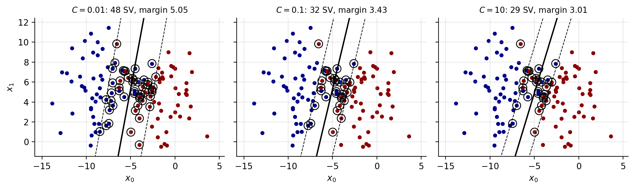
Figure 6.2: Soft-margin solutions for three values of \(C\) on overlapping classes. Circled points are support vectors. Decreasing \(C\) widens the margin and admits more violations, in accordance with the three KKT cases of Section The soft margin.
6.7. Kernels and non-linearity#
Everything so far produces a linear boundary. As in Section The linear model and the design matrix, we can gain flexibility by expanding the features – replacing \(\bm{x}\) by \(\bm{z}=\phi(\bm{x})\) for some map \(\phi\) into a higher-dimensional space, and separating linearly there. A boundary that is linear in \(\bm{z}\) is curved in \(\bm{x}\).
The simplest illustration is one-dimensional. Take nine points on a line with the two outer groups in one class and the middle group in the other; no single threshold separates them. Now map \(x\mapsto(x,x^{2})\) into the plane. The points lie on a parabola, and a horizontal line at the right height separates them perfectly.
import numpy as np
import matplotlib.pyplot as plt

X1D = np.linspace(-4, 4, 9).reshape(-1, 1)
X2D = np.c_[X1D, X1D**2]                     # the map phi(x) = (x, x^2)
y = np.array([0, 0, 1, 1, 1, 1, 1, 0, 0])

fig, ax = plt.subplots(1, 2, figsize=(11, 4))
ax[0].plot(X1D[y == 0], np.zeros(4), "bs")
ax[0].plot(X1D[y == 1], np.zeros(5), "g^")
ax[0].set_xlabel(r"$x_1$"); ax[0].set_yticks([]); ax[0].axhline(0, color="k")

ax[1].plot(X2D[y == 0, 0], X2D[y == 0, 1], "bs")
ax[1].plot(X2D[y == 1, 0], X2D[y == 1, 1], "g^")
ax[1].plot([-4.5, 4.5], [6.5, 6.5], "r--", linewidth=3)   # the separating line
ax[1].set_xlabel(r"$x_1$"); ax[1].set_ylabel(r"$x_2$")
plt.show()
The problem with doing this literally. Suppose we work in two dimensions and choose the quadratic map
writing \(\bm{x}=(x,y)\) for a single sample. The dual objective (6.17) becomes
identical in form, with the constraints and the recovery of \(b\) unchanged. The only new work is computing \(\bm{z}_i^{T}\bm{z}_j\). Doing that literally means constructing every \(\phi(\bm{x}_i)\) and taking inner products in the larger space – feasible here, prohibitive for a map into a thousand dimensions, and impossible for one into infinitely many.
The kernel trick. Define the kernel
For the map (6.28) we can evaluate it explicitly,
the last step by recognising the expansion of a square. This is the whole idea. The inner product in the three-dimensional feature space is a function of the inner product in the original two-dimensional space. We never construct \(\phi\); we compute \((\bm{x}_i^{T}\bm{x}_j)^{2}\) directly, at the cost of a two-dimensional dot product and one multiplication.
Replacing every inner product by a kernel, the dual becomes
with the same constraints (6.26), and the classifier Eq. (6.22) becomes
Note what has not survived: \(\bm{w}\) itself. It lives in the feature space and may be infinite-dimensional, so we never form it; the sum over support vectors in Eq. (6.33) is the only representation we have or need. This is why the dual formulation was worth the effort. The matrix in Eq. (6.20) simply acquires entries \(P_{ij}=y_iy_jK(\bm{x}_i,\bm{x}_j)\).
6.7.1. Common kernels and Mercer’s theorem#
Several kernels are in common use:
Linear: \(K(\bm{x},\bm{y})=\bm{x}^{T}\bm{y}\).
Polynomial: \(K(\bm{x},\bm{y})=(\gamma\,\bm{x}^{T}\bm{y}+r)^{d}\).
Gaussian radial basis function: \(K(\bm{x},\bm{y})=\exp\left(-\gamma\|\bm{x}-\bm{y}\|^{2}\right)\).
Sigmoid: \(K(\bm{x},\bm{y})=\tanh(\gamma\,\bm{x}^{T}\bm{y}+r)\).
A natural worry is whether an arbitrary function of two arguments corresponds to any feature map at all. Mercer’s theorem answers it: if \(K\) is symmetric, continuous, and such that the matrix with entries \(K(\bm{x}_i,\bm{x}_j)\) is positive semi-definite for every finite set of points, then there exists a map \(\phi\), possibly into a space of very high or infinite dimension, with \(K(\bm{x}_i,\bm{x}_j)=\phi(\bm{x}_i)^{T}\phi(\bm{x}_j)\). We may therefore use \(K\) knowing that \(\phi\) exists, without ever knowing what it is. Some frequently used kernels – the sigmoid among them – fail Mercer’s conditions for some parameter values and nevertheless work acceptably in practice.
The Gaussian kernel deserves a remark, because it is the default choice and its feature map is infinite-dimensional. Expanding the exponential in a power series produces terms of every polynomial degree, so the RBF kernel corresponds to a map into a space containing all monomials, with the higher-order ones progressively down-weighted. The parameter \(\gamma\) sets the length scale over which two points are considered similar: a large \(\gamma\) makes \(K\) decay rapidly, so each support vector influences only its immediate neighbourhood and the boundary becomes highly flexible; a small \(\gamma\) makes the kernel nearly constant and the boundary nearly linear. Together with \(C\) this gives two hyperparameters, and they interact, so the cross-validated search of Section Cross-validation should be a two-dimensional grid.
Machine learning connection
The kernel matrix \(K_{ij}=K(\bm{x}_i,\bm{x}_j)\) is the Gram matrix met in Section The covariance matrix, and its positive semi-definiteness is the same condition that made covariance matrices well behaved. The same object underlies Gaussian process regression, where the Cholesky factorisation of Section LU and Cholesky decompositions is applied to \(\bm{K}+\sigma^{2}\bm{I}\), and kernel ridge regression, which is Ridge regression with inner products replaced by kernels in exactly the manner of this section. A word of caution about cost: the kernel matrix has \(n^{2}\) entries and most solvers need \(\bigO(n^{2})\) to \(\bigO(n^{3})\) operations, so kernel methods scale badly in the number of samples even while scaling beautifully in the number of features. For \(n\) beyond a few tens of thousands one turns to linear SVMs solved in the primal, as in Section The primal view: the hinge loss, or to approximations of the kernel map.
Figure 6.3 shows the same data separated by three kernels. The linear kernel cannot represent the crescent boundary and misclassifies a large fraction; the cubic polynomial and the Gaussian both succeed, the latter producing a boundary that follows the data closely. Note the support vector counts printed above each panel: the polynomial kernel achieves the higher accuracy with twenty support vectors while the Gaussian needs more than twice as many, which by the argument of Section The soft margin suggests the polynomial model is the better matched of the two.
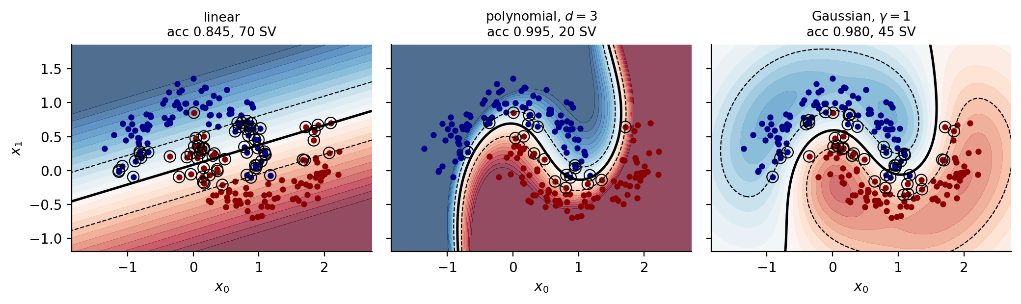
Figure 6.3: Decision functions for three kernels on the moons data, all fitted with the solver of Section Implementation. Solid contour: the boundary; dashed: the \(\pm1\) margins; circles: support vectors. Colour shows the value of Eq. (6.33) before the sign is taken.
6.8. The quadratic programme#
Collecting the results, the problem we must solve is
with \(P_{ij}=y_iy_jK(\bm{x}_i,\bm{x}_j)\), \(\bm{q}=-\mathbb{1}\), \(\bm{A}=\bm{y}^{T}\) and \(f=0\). The box constraints (6.26) split into \(-\lambda_i\le0\) and \(\lambda_i\le C\), which stacked together give
This is a quadratic programme: a convex quadratic objective with linear constraints, the class of problems treated at length by Boyd and Vandenberghe [boyd2004].
One could hand Eq. (6.34) to a general-purpose quadratic
programming package – CVXOPT is the usual choice in Python – and
many treatments stop there. We shall not, for two reasons. A general solver
treats \(\bm{P}\) as a dense \(n\times n\) matrix and costs \(\bigO(n^{3})\), which
is wasteful given the very special structure here. And, more importantly, the
algorithm that exploits that structure is simple enough to derive completely,
which is worth more than a library call.
Why gradient descent will not do. It is worth being explicit about why Chapter 4 does not simply apply. A gradient step moves \(\bm{\lambda}\) in an arbitrary direction and will in general violate both \(0\le\lambda_i\le C\) and \(\sum_i\lambda_iy_i=0\). One could project back onto the feasible set after each step – projected gradient descent – but the projection onto the intersection of a box and a hyperplane is itself a small optimisation problem. The algorithm below takes a cleverer route: it moves in directions that preserve feasibility by construction.
6.9. Sequential minimal optimisation#
The key observation is due to Platt. The equality constraint \(\sum_i\lambda_iy_i=0\) couples all the multipliers, so we cannot change one alone without violating it. But we can change two at once, adjusting the second to compensate the first. Two is therefore the smallest possible working set, and the resulting subproblem – a quadratic in one effective variable – can be solved analytically. No inner numerical optimisation is needed anywhere. Hence the name: sequential minimal optimisation.
The subproblem. Fix all multipliers except \(\lambda_1\) and \(\lambda_2\). The equality constraint requires
a constant. Multiplying by \(y_1\) and using \(y_1^{2}=1\),
so the pair is confined to a line, and the problem has one free variable.
The bounds. Feasibility requires both multipliers to lie in \([0,C]\), which restricts \(\lambda_2\) to an interval \([L,H]\) determined by the geometry of the line and the box. Two cases arise. If \(y_1\ne y_2\) then \(s=-1\) and Eq. (6.37) gives \(\lambda_1-\lambda_2=\gamma\), a line of slope \(+1\); requiring both coordinates to lie in \([0,C]\) gives
If \(y_1=y_2\) then \(s=+1\) and \(\lambda_1+\lambda_2=\gamma\), a line of slope \(-1\), giving
If \(L=H\) the line meets the box in a single point and there is nothing to do.
The analytic solution. Substituting Eq. (6.37) into the dual objective (6.32) gives a quadratic in \(\lambda_2\) alone. Writing \(K_{ij}=K(\bm{x}_i,\bm{x}_j)\), its second derivative is
which is \(\le0\) because \(K_{11}-2K_{12}+K_{22}=\|\phi(\bm{x}_1)-\phi(\bm{x}_2)\|^{2}\ge0\) by Eq. (6.30). The objective is therefore concave along the line and has a unique maximum. Setting the first derivative to zero and expressing the result in terms of the prediction errors
the unconstrained maximiser is
Since \(\eta<0\), the step moves \(\lambda_2\) opposite to \(y_2(E_1-E_2)\), which is the direction of increasing \(\mathcal{L}\). Clipping to the feasible interval,
and recovering the partner from Eq. (6.37),
The equality constraint is satisfied exactly, by construction, at every step.
Updating the intercept. After each step \(b\) must be recomputed so that the KKT conditions (6.27) hold for the two points just changed. If \(\lambda_1^{\mathrm{new}}\) lies strictly inside \((0,C)\) then point \(1\) is a free support vector and must satisfy \(y_1f(\bm{x}_1)=1\), which gives
and symmetrically for point \(2\),
If both multipliers are free the two agree; if only one is free we use the corresponding value; if neither is free any value between them satisfies the conditions and we take the average.
Choosing the pair. What remains is a heuristic for selecting which two multipliers to optimise, and here we are guided by the KKT conditions rather than by the objective. Define \(r_i=y_iE_i\). The conditions of Section The soft margin are violated when
for a tolerance \(\epsilon\). The outer loop alternates between sweeping all points and sweeping only the free support vectors – the latter being where the action is, since bound multipliers tend to stay bound – and terminates when a full sweep over all points produces no change, at which point the KKT conditions hold everywhere and we have the solution. Given a violating \(i\), the second index \(j\) is chosen to maximise \(|E_i-E_j|\), since by Eq. (6.42) the step length is proportional to that difference.
6.10. Implementation#
We now write the solver. It is short, it uses nothing beyond
numpy, and every line corresponds to an equation above.
import numpy as np


def linear_kernel(X, Z):
    return X @ Z.T


def polynomial_kernel(X, Z, degree=3, gamma=1.0, coef0=1.0):
    return (gamma * (X @ Z.T) + coef0) ** degree


def rbf_kernel(X, Z, gamma=1.0):
    """Gaussian kernel, computed through the identity
    ||x - z||^2 = ||x||^2 + ||z||^2 - 2 x.z  (Section 1.vectors)."""
    d2 = (np.sum(X**2, axis=1)[:, None] + np.sum(Z**2, axis=1)[None, :]
          - 2.0 * (X @ Z.T))
    return np.exp(-gamma * np.maximum(d2, 0.0))
The kernel matrix is computed once and cached, as are the errors \(E_i\); both are the standard economies.
class SVC:
    """Support vector classifier trained by sequential minimal optimisation.

    Solves the dual (6.dualkernel) subject to the box constraints
    (6.boxconstraints), using the analytic two-variable update (6.smoupdate).
    Labels must be -1 and +1.
    """

    def __init__(self, C=1.0, kernel=linear_kernel, tol=1e-4, max_iter=10000):
        self.C = C
        self.kernel = kernel
        self.tol = tol
        self.max_iter = max_iter

    # ---------- the two-variable subproblem ----------
    def _take_step(self, i, j):
        if i == j:
            return False
        C, lam, y, K, E = self.C, self.lam_, self.y_, self.K_, self.E_
        li, lj = lam[i], lam[j]

        # Bounds L and H, Eqs. (6.boundsdiff) and (6.boundssame)
        if y[i] != y[j]:
            L, H = max(0.0, lj - li), min(C, C + lj - li)
        else:
            L, H = max(0.0, li + lj - C), min(C, li + lj)
        if L >= H:
            return False

        eta = 2.0 * K[i, j] - K[i, i] - K[j, j]        # Eq. (6.eta)
        if eta >= -1e-12:                              # degenerate, skip
            return False

        lj_new = lj - y[j] * (E[i] - E[j]) / eta       # Eq. (6.smoupdate)
        lj_new = min(H, max(L, lj_new))                # Eq. (6.clip)
        if abs(lj_new - lj) < 1e-10 * (lj_new + lj + 1e-10):
            return False
        li_new = li + y[i] * y[j] * (lj - lj_new)      # Eq. (6.smopartner)

        b1 = (self.b_ - E[i] - y[i] * (li_new - li) * K[i, i]
              - y[j] * (lj_new - lj) * K[i, j])        # Eq. (6.b1)
        b2 = (self.b_ - E[j] - y[i] * (li_new - li) * K[i, j]
              - y[j] * (lj_new - lj) * K[j, j])        # Eq. (6.b2)
        if 1e-8 < li_new < C - 1e-8:
            b_new = b1
        elif 1e-8 < lj_new < C - 1e-8:
            b_new = b2
        else:
            b_new = 0.5 * (b1 + b2)

        lam[i], lam[j] = li_new, lj_new
        self.b_ = b_new
        self.E_ = (self.K_ @ (lam * y)) + self.b_ - y   # refresh the cache
        return True

    # ---------- choose the partner for a violating index ----------
    def _examine(self, i):
        y, lam, C = self.y_, self.lam_, self.C
        r = y[i] * self.E_[i]
        violates = ((r < -self.tol and lam[i] < C - 1e-12) or
                    (r > self.tol and lam[i] > 1e-12))   # Eq. (6.kktviolation)
        if not violates:
            return False

        free = np.where((lam > 1e-12) & (lam < C - 1e-12))[0]
        if len(free) > 1:                       # heuristic: maximise |E_i - E_j|
            j = free[np.argmax(np.abs(self.E_[i] - self.E_[free]))]
            if self._take_step(i, j):
                return True
        for j in np.random.permutation(free):   # then any free multiplier
            if self._take_step(i, j):
                return True
        for j in np.random.permutation(len(y)):  # then anything at all
            if self._take_step(i, j):
                return True
        return False

    # ---------- the outer loop ----------
    def fit(self, X, y):
        X = np.asarray(X, dtype=float)
        y = np.asarray(y, dtype=float)
        n = len(y)

        self.X_, self.y_ = X, y
        self.K_ = self.kernel(X, X)
        self.lam_ = np.zeros(n)
        self.b_ = 0.0
        self.E_ = -y.copy()                    # since lambda = 0 and b = 0

        examine_all, num_changed, it = True, 0, 0
        while (num_changed > 0 or examine_all) and it < self.max_iter:
            num_changed = 0
            if examine_all:
                index_set = range(n)
            else:                              # only the free support vectors
                index_set = np.where((self.lam_ > 1e-12)
                                     & (self.lam_ < self.C - 1e-12))[0]
            for i in index_set:
                num_changed += self._examine(i)
                it += 1
            if examine_all:
                examine_all = False
            elif num_changed == 0:
                examine_all = True

        sv = self.lam_ > 1e-8
        self.sv_ = sv
        self.X_sv, self.y_sv, self.lam_sv = X[sv], y[sv], self.lam_[sv]
        self.n_iter_ = it
        return self

    def decision_function(self, X):
        """Eq. (6.kernelclassify) without the sign."""
        X = np.asarray(X, dtype=float)
        return self.kernel(X, self.X_sv) @ (self.lam_sv * self.y_sv) + self.b_

    def predict(self, X):
        return np.sign(self.decision_function(X))
Note that \(\bm{w}\) never appears. For a linear kernel it can be recovered
from Eq. (6.16) as (lam_sv * y_sv) @ X_sv, but
for the RBF kernel it does not exist as a finite vector and the sum over
support vectors in decision_function is the only representation
available.
6.11. Verifying the solver#
A solver written from scratch must be checked, and the KKT conditions give us exactly the tests to apply. Rather than merely comparing predictions against a library, we verify the mathematics.
import numpy as np
from sklearn.datasets import make_blobs, make_moons
from sklearn.svm import SVC as SklearnSVC

np.random.seed(0)

# --- a separable linear problem ---
X, y01 = make_blobs(n_samples=80, centers=2, cluster_std=0.8, random_state=3)
y = np.where(y01 == 0, -1.0, 1.0)

model = SVC(C=10.0, kernel=linear_kernel).fit(X, y)
w = (model.lam_sv * model.y_sv) @ model.X_sv            # Eq. (6.wfromlambda)

reference = SklearnSVC(C=10.0, kernel="linear").fit(X, y)
print("ours    w =", np.round(w, 5), " b =", round(model.b_, 5))
print("sklearn w =", np.round(reference.coef_.ravel(), 5),
      " b =", round(reference.intercept_[0], 5))
The two agree to about \(3\times10^{-4}\) in \(\bm{w}\) and \(8\times10^{-4}\) in \(b\), the difference being the finite KKT tolerance. More telling is the direct check of the conditions themselves.
X, y01 = make_moons(n_samples=200, noise=0.15, random_state=42)
y = np.where(y01 == 0, -1.0, 1.0)

gaussian = lambda A, B: rbf_kernel(A, B, gamma=1.0)
model = SVC(C=1.0, kernel=gaussian).fit(X, y)

margin = y * model.decision_function(X)                 # y_i f(x_i)
lam = model.lam_
free = (lam > 1e-6) & (lam < model.C - 1e-6)

print(f"free support vectors: |y f - 1| max = "
      f"{np.abs(margin[free] - 1).max():.2e}")          # must be 0
print(f"lambda = 0 points:    min y f = {margin[lam <= 1e-8].min():.4f}")  # >= 1
print(f"equality constraint:  sum lam y = {np.sum(lam * y):.2e}")          # = 0

dual = np.sum(lam) - 0.5 * np.sum(np.outer(lam * y, lam * y) * model.K_)
print(f"dual objective: {dual:.6f}")
The output is
free support vectors: |y f - 1| max = 8.95e-05
lambda = 0 points:    min y f = 1.0002
equality constraint:  sum lam y = -8.88e-16
dual objective: 27.790313
Every condition of Section The soft margin holds. The free support
vectors sit on the margin to five decimal places; the points with vanishing
multipliers all satisfy \(y_if(\bm{x}_i)\ge1\), so none has been wrongly
excluded; and the equality constraint holds to machine precision, as it must,
since Eq. (6.44) enforces it exactly at every step. The dual
objective agrees with the value \(27.790310\) obtained from
scikit-learn’s multipliers to six significant figures – our value
being very slightly the larger, as it should be for a maximisation. On this
data set both classifiers reach \(98\%\) training accuracy and agree on every
single prediction.
The soft margin in action. Repeating on deliberately overlapping classes shows what \(C\) controls.
X, y01 = make_blobs(n_samples=120, centers=2, cluster_std=2.6, random_state=7)
y = np.where(y01 == 0, -1.0, 1.0)

for C in [0.01, 0.1, 1.0, 10.0]:
    m = SVC(C=C, kernel=linear_kernel).fit(X, y)
    w = (m.lam_sv * m.y_sv) @ m.X_sv
    at_bound = int(np.sum(m.lam_ > C - 1e-6))
    print(f"C={C:<6} n_sv={m.sv_.sum():3d} (at bound {at_bound:3d})  "
          f"margin={2/np.linalg.norm(w):7.4f}  "
          f"accuracy={np.mean(m.predict(X) == y):.4f}")
C=0.01   n_sv= 48 (at bound  46)  margin= 5.0478  accuracy=0.8750
C=0.1    n_sv= 32 (at bound  29)  margin= 3.4275  accuracy=0.8833
C=1.0    n_sv= 29 (at bound  26)  margin= 3.0133  accuracy=0.8833
C=10.0   n_sv= 28 (at bound  25)  margin= 2.9851  accuracy=0.8833
The support vector counts match scikit-learn exactly for every \(C\).
Reading the table, a small \(C\) makes violations cheap, so many points sit
inside a wide margin and most multipliers are at the bound; increasing \(C\)
raises the price of a violation, so the margin narrows and fewer points
support it. The training accuracy barely moves, because these classes
genuinely overlap and no linear boundary can do better – which is the
situation the soft margin was invented for.
One caveat about reproducibility. The partner-selection heuristic of
Section Sequential minimal optimisation falls back on a random permutation when the free
multipliers offer no improvement, so the iterate path – and hence the last
few digits of the margin, and occasionally the count of bound multipliers by
one – depends on the seed. The solution itself does not: the dual objective
and the predictions are reproducible, because the problem is convex and the
optimum unique. The table above was produced with np.random.seed(0)
set immediately before the loop.
The kernel trick, verified. The identity (6.31) can be checked directly.
rng = np.random.default_rng(1)
a, b = rng.normal(size=2), rng.normal(size=2)
phi = lambda v: np.array([v[0]**2, v[1]**2, np.sqrt(2) * v[0] * v[1]])

print(phi(a) @ phi(b), (a @ b)**2)      # 0.9148995105  0.9148995105
On the moons data a cubic polynomial kernel with \(C=5\) reaches \(99.5\%\)
training accuracy with only \(20\) support vectors, identical to
scikit-learn in both figures – a more compact model than the RBF
kernel needed, because the true boundary happens to be well matched by a
low-order polynomial.
6.12. The primal view: the hinge loss#
The dual is not the only route, and the alternative reveals what a support vector machine has in common with everything else in this book.
Return to the soft-margin problem. For a given \((\bm{w},b)\) the optimal slack is as small as Eq. (6.23) permits, namely \(\xi_i=\max\left(0,\,1-y_i(\bm{w}^{T}\bm{x}_i+b)\right)\). Substituting this into the primal objective eliminates the slack variables and leaves an unconstrained problem,
where \(\lambda\) is proportional to \(1/C\). The function \(\max(0,1-y f)\) is the hinge loss: zero once the point is correctly classified with margin at least one, and growing linearly thereafter.
Equation (6.48) should look familiar. It is a loss plus an \(\ell_2\) penalty – precisely the structure of Ridge regression in Eq. (3.43) and of penalised logistic regression in Eq. (5.23). The three methods differ only in the loss:
Method |
Loss on one sample |
|---|---|
Ridge regression |
\(\left(y_i-f_i\right)^{2}\) |
Logistic regression |
\(\log\left(1+e^{-y_if_i}\right)\) |
Support vector machine |
\(\max\left(0,\,1-y_if_i\right)\) |
with \(f_i=\bm{w}^{T}\bm{x}_i+b\) throughout, and the labels \(\pm1\) in the last two rows. Comparing the second and third explains the difference in behaviour. The logistic loss is positive everywhere, however well a point is classified, so every point exerts some pull on the boundary – which is why logistic regression has no support vectors. The hinge loss is exactly zero beyond the margin, so points that are comfortably correct exert none at all – which is why the SVM does. This is the same fact we derived from the KKT conditions in Section The dual problem, now visible in the loss function itself.
Figure 6.4 draws the three losses of the table together with the misclassification loss they are all trying to approximate. All three are convex upper bounds on the step function, which is what makes them tractable surrogates. They differ in two respects that matter. Only the hinge loss is exactly zero for \(yf>1\), which produces the support vectors; and the squared loss is the only one that increases for large positive margin, penalising a point for being classified too well, which is why it is a poor choice for classification.
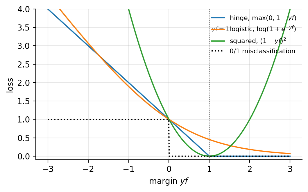
Figure 6.4: The hinge, logistic and squared losses as functions of the margin \(yf\), with the \(0/1\) misclassification loss they bound. Only the hinge vanishes identically beyond \(yf=1\); only the squared loss grows again for large positive margin.
Solving the primal directly. Because Eq. (6.48) is unconstrained, the methods of Chapter 4 apply after all. The hinge is not differentiable at the kink, but it is convex and possesses a subgradient everywhere, which is enough. The resulting algorithm, Pegasos, is stochastic gradient descent with the learning rate schedule \(\gamma_t=1/(\lambda t)\) of Eq. (4.35).
import numpy as np

def pegasos(X, y, lmbda=0.01, epochs=300, rng=None):
    """Primal SVM by stochastic subgradient descent on Eq. (6.hingeobjective)."""
    rng = np.random.default_rng(0) if rng is None else rng
    n, p = X.shape
    w, b, t = np.zeros(p), 0.0, 0
    for _ in range(epochs):
        for i in rng.permutation(n):
            t += 1
            gamma = 1.0 / (lmbda * t)                  # Eq. (4.timedecay)
            if y[i] * (w @ X[i] + b) < 1:            # inside the margin
                w = (1 - gamma * lmbda) * w + gamma * y[i] * X[i]
                b += gamma * y[i]
            else:                                    # outside: only the penalty
                w = (1 - gamma * lmbda) * w
    return w, b
On the standardised overlapping blobs above with \(\lambda=0.01\), Pegasos
reaches an objective of \(0.255097\) against \(0.255064\) for the dual solution
computed by scikit-learn – agreement to four decimal places – with
identical training accuracy. The two formulations solve the same problem.
Which to prefer is decided by the shape of the data, and the criterion is the one that has recurred throughout this book. The dual has \(n\) variables and needs the \(n\times n\) kernel matrix, so it suits problems with few samples, many features, and a non-linear boundary. The primal has \(p+1\) variables and touches one sample at a time, so it suits problems with very many samples and a linear boundary. For text classification with a million documents and a million features, Pegasos is the practical choice and the kernel matrix is unthinkable.
Machine learning connection
The table above is worth memorising, because it organises a large part of supervised learning. Fix the model \(f=\bm{w}^{T}\bm{x}+b\) and the penalty \(\|\bm{w}\|^{2}\), and the choice of loss selects the method: squared error gives Ridge, log loss gives logistic regression, hinge loss gives the SVM. Change the penalty from \(\ell_2\) to \(\ell_1\) and each acquires a sparse variant, as in Section The Lasso. Replace the linear \(f\) by a neural network and the same losses reappear unchanged in the next chapters. The apparent variety of methods is largely a small number of choices made independently, and recognising which choice a new method is making is usually the fastest way to understand it.
6.13. One penalty, three losses#
Section The primal view: the hinge loss ended by placing the support vector machine in a family: Ridge regression, logistic regression and the support vector machine are one model with one penalty and three losses. That remark was about linear models. It survives the kernel trick intact, and in the kernel setting it becomes sharper, because it explains the one property that distinguishes this chapter’s method from the other two – sparsity – and shows that the property is a consequence of the loss function alone.
6.13.1. The common problem#
All three methods solve
over the reproducing kernel Hilbert space of Section Why the same trick works for any loss: the representer theorem, and differ only in \(L\). With labels \(y_i\in\{-1,+1\}\) as in this chapter:
By Theorem 3.12 all three minimisers have the form \(f=\sum_j\alpha_jk(\bm{x}_j,\cdot)\), so all three produce a prediction rule of exactly the shape (6.33). The only thing that can distinguish them is the vector \(\bm{\alpha}\), and there is a single formula for it.
Theorem 6.1 (The coefficients are minus the loss derivative)
Let \(f^{\star}\) minimise Eq. (6.49) with \(L\) convex and differentiable in its second argument, and write \(L'_i=\partial L(y_i,f)/\partial f\) evaluated at \(f=f^{\star}(\bm{x}_i)\). Then
If \(L\) is convex but not differentiable, the same holds with \(L'_i\) any element of the subdifferential \(\partial L(y_i,f^{\star}(\bm{x}_i))\), in the sense of Eq. (3.65).
Proof
By the reproducing property, \(f\mapsto f(\bm{x}_i)\) has derivative \(k(\bm{x}_i,\cdot)\) as an element of \(\mathcal{H}\): perturbing \(f\) by \(\delta\) changes \(f(\bm{x}_i)\) by \(\langle\delta,k(\bm{x}_i,\cdot)\rangle\). The derivative of \(\tfrac{\lambda}{2}\|f\|^{2}\) is \(\lambda f\). Stationarity of Eq. (6.49) in \(\mathcal{H}\) is therefore
which rearranges to Eq. (6.53). For non-differentiable \(L\) the same argument applies with the subdifferential, \(0\) belonging to the sum of the subdifferential of the loss and the gradient of the penalty. \qed
Equation (6.53) is short and it settles everything. The weight a training point receives in the final predictor is the derivative of the loss at that point, divided by the penalty. A point on which the loss is locally flat receives no weight at all. Applying it in turn:
Squared loss. \(L'=f-y\), so \(\alpha_i=(y_i-f_i)/\lambda\): the coefficient is the residual. Substituting into \(\bm{f}=\bm{K}\bm{\alpha}\) gives \(\bm{K}\bm{\alpha}=\bm{y}-\lambda\bm{\alpha}\), that is \((\bm{K}+\lambda\bm{I})\bm{\alpha}=\bm{y}\), which is Eq. (3.84) – the theorem contains kernel ridge regression as a special case.
Logistic loss. \(L'=-y\,\sigma(-yf)\), so \(\alpha_i=y_i\sigma(-y_if_i)/\lambda\). For labels in \(\{0,1\}\) this is Proposition 5.2, \(\alpha_i=(y_i-p_i)/\lambda\), in the other notation. The logistic function is strictly positive everywhere, so no coefficient vanishes.
Hinge loss. \(L'=-y\) where \(yf<1\) and \(L'=0\) where \(yf>1\), so
The hinge loss is the only one of the three that is exactly zero on an open set, so its derivative is exactly zero there, so its coefficients are exactly zero there. That is the entire origin of the support vectors. The points with \(\alpha_i\neq0\) are precisely those with \(y_if_i\le1\) – inside the margin or misclassified – which is the characterisation Section The dual problem obtained from the Karush-Kuhn-Tucker conditions, and the bound \(y_i\alpha_i\le1/\lambda\) is the box constraint \(\lambda_i\le C\) of Eq. (6.26) with \(C=1/\lambda\).
6.13.2. The three, measured together#
The program \verb!three_losses.py! fits all three to the same eighty points with the same Gaussian kernel and the same \(\lambda=1\), and checks Eq. (6.53) directly. The hinge problem is solved as the box-constrained quadratic programme obtained by writing \(\alpha_i=y_i\beta_i/\lambda\), which is the dual of Section The dual problem without the equality constraint, since Eq. (6.49) carries no unpenalised intercept; the solver certifies itself by the duality gap:
  primal value  26.4874425949
  dual value    26.4874425949
  duality gap   1.528e-13
The theorem then holds to machine precision for all three:
   loss          L'(y,f)                      predicted alpha        max |alpha - predicted|
   squared       f - y                        (y - f)/lambda        1.332e-15
   logistic      -y sigma(-y f)               y sigma(-y f)/lambda  1.468e-13
   hinge         -y if yf<1, 0 if yf>1        y/lambda or 0         0.000e+00
The hinge row excludes the fifteen points lying exactly on the margin, where \(L\) is not differentiable and Eq. (6.55) permits any value between \(0\) and \(y_i/\lambda\). Those points are not an inconvenience of the measurement; they are the reason the subdifferential appears in the statement of the theorem.
And here is the consequence the theorem predicts:
   method                    non-zero alpha   |alpha|_max   sum L(y_i,f_i)   (lambda/2)||f||^2   objective
   kernel ridge                         80        1.9253        10.738297            4.251415   14.989712
   kernel logistic                      80        0.8013        29.757767            7.832128   37.589895
   support vector machine               44        1.0000        17.979270            8.508173   26.487443
Eighty of eighty for the two smooth losses, forty-four of eighty for the hinge. The largest coefficient of the support vector machine is exactly \(1.0000=1/\lambda\), which is the upper bound in Eq. (6.55) attained at the misclassified points, and no such bound constrains the other two. Varying the penalty:
     lambda    SVM non-zeros   ridge non-zeros   logistic non-zeros
       0.10              24                  80                     80
       1.00              44                  80                     80
      10.00              79                  80                     80
     100.00              80                  80                     80
The sparsity of the support vector machine is not fixed but bought: a large penalty flattens \(f\), more points fall inside the margin \(y_if_i\le1\), and more coefficients switch on. In the limit of a very heavy penalty every point is a support vector and the advantage disappears entirely. The other two are dense at every penalty, as Theorem 6.1 says they must be.
Finally, the three fitted functions are not very different:
   method                    test accuracy   agreement with SVM
   kernel ridge                      0.9025               0.9800
   kernel logistic                   0.8760               0.9635
   support vector machine            0.8825               1.0000
Three methods, three losses, one penalty, one representation, decision boundaries agreeing on the large majority of the plane – and one of them built from a little over half the data. The choice among them is a choice of what to pay for: a closed form and a single linear solve (squared error), a calibrated probability (logistic), or a sparse predictor (hinge).
Machine learning connection
Theorem 6.1 is a good example of a result that is worth more than the sum of its applications. It says that in a kernel method the loss function does not merely decide how well the fit tolerates an error; it decides which observations appear in the answer at all. A loss that is flat somewhere yields a sparse representation, and one that is not, does not. That principle generalises beyond the three cases here – \(\epsilon\)-insensitive regression is flat in a band around zero and gives sparse support vectors for a regression problem, for exactly this reason – and it is a useful thing to know when reading a proposal for a new loss function. Ask where it is flat.
6.14. Summary and the programs#
The support vector machine begins from a geometric principle rather than a statistical one: among the separating hyperplanes, choose the one standing furthest from the data. Fixing the scale so that the nearest points satisfy \(y_i(\bm{w}^{T}\bm{x}_i+b)=1\) turns maximising the margin into minimising \(\tfrac12\|\bm{w}\|^{2}\) under linear inequality constraints, Eq. (6.8).
Lagrange duality then does something remarkable. Eliminating the primal variables produces Eq. (6.17), in which the data appear only through inner products, the number of variables is the number of samples, and the KKT conditions show that most multipliers vanish. The surviving points – the support vectors – are the only ones that matter; every other point could be deleted without changing the answer. Slack variables extend this to overlapping classes and, remarkably, change nothing in the dual but the addition of a ceiling \(\lambda_i\le C\).
Because only inner products appear, they can be replaced by a kernel, and Mercer’s theorem guarantees that any symmetric positive semi-definite kernel corresponds to some feature map. We thereby separate data linearly in a space we never construct, possibly of infinite dimension, at the cost of evaluating a function of two arguments.
The dual is a quadratic programme, and rather than call a library we derived
and built a solver. Sequential minimal optimisation exploits the fact that
the equality constraint forces multipliers to be changed in pairs, so the
smallest possible subproblem has two variables, one of them eliminated by the
constraint – and a one-dimensional concave quadratic can be maximised in
closed form, Eq. (6.42). The whole algorithm is analytic
updates plus a selection heuristic, it never needs a matrix factorisation, and
the implementation of Section Implementation reproduces
scikit-learn to six significant figures in the dual objective while
satisfying every KKT condition to five decimal places.
Finally, eliminating the slack variables in the primal revealed the hinge loss and placed the SVM in a family: Ridge regression, logistic regression and the support vector machine are one model with one penalty and three losses. The hinge loss is the only one of the three that is exactly zero for well-classified points, which is the entire origin of sparsity in the support vectors.
Section One penalty, three losses turned that remark into Theorem 6.1, which holds for the kernel forms of all three methods and gives the coefficients of any of them in one line, \(\alpha_i=-L'_i/\lambda\). The weight a training point carries is the derivative of the loss at that point. A loss that is flat on an open set has zero derivative there and therefore zero coefficients; the hinge is the only one of the three that is, and the support vectors follow. Measured on eighty points with the same kernel and the same penalty, the formula holds to between \(10^{-13}\) and machine zero for all three losses, the support vector machine retains forty-four coefficients and the other two retain all eighty, and the three decision boundaries agree on more than ninety-six per cent of the plane.
The complete programs are collected in doc/BookML/BookPrograms:
three_losses.py– kernel ridge regression, kernel logistic regression and the support vector machine fitted to the same data with the same kernel, the hinge problem solved as a box-constrained quadratic programme and certified by its duality gap, and Theorem 6.1 checked for all three.svm_smo.py– theSVCclass of Section Implementation with the linear, polynomial and Gaussian kernels, and the KKT verification of Section Verifying the solver.svm_examples.py– the separable blobs, the effect of \(C\) on overlapping classes, the moons data with polynomial and RBF kernels, and the decision-boundary plots.svm_pegasos.py– the primal subgradient solver of Section The primal view: the hinge loss, with the comparison of the primal and dual objectives.losses.py– the squared, logistic and hinge losses plotted together, reproducing the table of Section The primal view: the hinge loss.
Each file runs as a script and reproduces the numbers quoted in this chapter.
6.15. Exercises#
6.15.1. Warm-up exercises#
Geometry of the hyperplane. (a) Show that \(\bm{w}\) is orthogonal to the hyperplane \(\bm{w}^{T}\bm{x}+b=0\). (b) Derive the signed distance (6.2). (c) Show that the distance between the two margin hyperplanes \(\bm{w}^{T}\bm{x}+b=\pm1\) is \(2/\|\bm{w}\|\).
Scale invariance. Show that multiplying \((\bm{w},b)\) by any \(\alpha>0\) leaves the decision boundary unchanged, and explain why this licenses the normalisation used to obtain Eq. (6.8).
The dual, by hand. (a) Derive Eqs. (6.14) and (6.15) from the Lagrangian (6.13). (b) Substitute back and obtain the dual (6.17), being explicit about how the term in \(b\) disappears. (c) Show that the matrix \(P_{ij}=y_iy_j\bm{x}_i^{T}\bm{x}_j\) is positive semi-definite, and hence that the dual is convex.
A two-point problem. Take \(\bm{x}_1=(0,0)\) with \(y_1=-1\) and \(\bm{x}_2=(2,0)\) with \(y_2=+1\). (a) Write out the dual and solve it by hand for \(\lambda_1\) and \(\lambda_2\). (b) Recover \(\bm{w}\) and \(b\), and verify that the margin is \(2/\|\bm{w}\|\) and equals the distance between the points. (c) Confirm your answer with the code of Section Implementation.
The three KKT cases. For the soft-margin problem, derive the classification of points into \(\lambda_i=0\), \(0<\lambda_i<C\) and \(\lambda_i=C\) given at the end of Section The soft margin, starting from Eqs. (6.27) and \(\lambda_i=C-\gamma_i\).
The SMO bounds. (a) Derive Eqs. (6.38) and (6.39) by drawing the box \([0,C]^{2}\) and the line \(\lambda_1=\gamma-s\lambda_2\) for both signs of \(s\). (b) Show that \(\eta=2K_{12}-K_{11}-K_{22}\le0\) for any valid kernel, and identify the case in which it vanishes. (c) What should the algorithm do when \(L=H\), and why?
The kernel trick. (a) Verify Eq. (6.31) algebraically. (b) Find the feature map corresponding to \(K(\bm{x},\bm{z})=(\bm{x}^{T}\bm{z}+1)^{2}\) in two dimensions, and count its dimensions. (c) Show that if \(K_1\) and \(K_2\) are valid kernels then so are \(K_1+K_2\) and \(K_1K_2\). (d) Show that the Gaussian kernel can be written as \(\exp(-\gamma\|\bm{x}\|^{2})\exp(-\gamma\|\bm{z}\|^{2}) \exp(2\gamma\bm{x}^{T}\bm{z})\) and, by expanding the last factor, argue that its feature space is infinite-dimensional.
Implementing SMO (numerical). Starting from the code of Section Implementation: (a) reproduce the KKT checks of Section Verifying the solver; (b) replace the max-\(|E_i-E_j|\) heuristic by a random choice of \(j\) and compare the number of iterations to convergence; (c) remove the alternation between sweeping all points and sweeping only the free multipliers, and report what happens to the dual objective.
Hyperparameters (numerical). On the moons data, perform a two-dimensional cross-validated grid search over \(C\) and the RBF \(\gamma\). (a) Plot the validation accuracy as a heat map. (b) Plot the number of support vectors over the same grid, and comment on the relation between that number and the generalisation error. (c) Show the decision boundary for a badly chosen and a well chosen pair.
The three losses. Plot the squared, logistic and hinge losses of Section The primal view: the hinge loss against the margin \(yf\) on the same axes. (a) Which are zero for large positive margin? (b) Which grow fastest for large negative margin, and what does that imply about sensitivity to outliers and mislabelled points? (c) Relate your answer to the notebox on the squared error in Section Maximum likelihood and the cross-entropy.
6.15.2. Project-style exercise: building a support vector machine#
Part a: the linear separable case. Implement the hard-margin SVM by writing the dual and solving it with your own SMO, taking \(C\) very large. Test on two well-separated Gaussian blobs. Plot the decision boundary, both margin hyperplanes, and the support vectors circled. Verify that exactly the circled points have \(\lambda_i>0\), and that deleting any other point leaves the solution unchanged – this last check is the definition of a support vector and is worth performing explicitly.
Part b: the soft margin. Move the blobs together until they overlap. Sweep \(C\) over several orders of magnitude and, for each, record the margin, the number of free and bound support vectors and the training accuracy. Explain the trends using the three KKT cases of Section The soft margin.
Part c: kernels. Add the polynomial and Gaussian kernels and apply them to the moons data and to a set of concentric circles. For the circles, find analytically a feature map making the problem linearly separable, and check that a polynomial kernel of the corresponding degree succeeds.
Part d: model selection. Cross-validate over \(C\) and \(\gamma\) as in Section Cross-validation, using a proper training, validation and test split. Report the confusion matrix and the metrics of Section Measuring the quality of a classifier on a test set used once.
Part e: comparison. On the Wisconsin breast cancer data of Section The Wisconsin breast cancer data, compare your SVM against the logistic regression of Chapter 5. Compare accuracy, AUC, the number of support vectors, and the training time. Which would you deploy, and why? Note that the SVM produces no probabilities; discuss what is lost thereby and what could be done about it.
Part f: primal against dual. Implement Pegasos as in Section The primal view: the hinge loss and verify that it reaches the same objective as your dual solver on a linear problem. Then time both as the number of samples grows from \(10^{2}\) to \(10^{5}\), and as the number of features grows over the same range. Plot the two scalings and identify the regime in which each formulation should be preferred.