
15. Chapter 15: Variational Autoencoders#
Two chapters have now approached generative modelling from opposite ends and each hit the same wall. Chapter 12 built an autoencoder that compressed data beautifully but was not a probability model at all: nothing in Eq. (12.2) says what the code \(\bm{z}\) should be distributed like, so sampling a code and decoding it produces nothing in particular. Chapter 14 built a genuine probability model whose likelihood was blocked by an intractable partition function, and spent itself on Markov chains to get around that.
The variational autoencoder takes a third route. It keeps the encoder-decoder architecture of Chapter 12 but makes both halves probability distributions, and it defeats the intractable likelihood not by sampling from the model, as in Chapter 14, but by optimising a computable lower bound on it. The bound is called the evidence lower bound, or ELBO, and deriving it, understanding when it is tight, and making it differentiable are the three things this chapter does.
The result is a model that is a real probability distribution, can be sampled in a single pass with no Markov chain, and trains by ordinary stochastic gradient descent. It also has two characteristic failures – blurry samples and posterior collapse – both of which follow from the objective rather than from bad luck, and both of which we measure. The chapter ends by showing how stacking the construction leads directly to the diffusion models of Chapter 16.
The material follows the lecture notes for weeks thirteen to fifteen of FYS-STK3155/4155 and the original account by Kingma and Welling [kingma2019].
15.1. The latent-variable model#
The model is the probabilistic PCA of Section The probabilistic view: PPCA with the linear map replaced by a network. A latent variable \(\bm{h}\in\mathbb{R}^{d_h}\) is drawn from a fixed prior, and the observation is drawn from a conditional whose parameters a network computes:
with \(p_{\bm{\theta}}(\bm{x}\mid\bm{h})\) Gaussian for continuous data or factorised Bernoulli for binary data, its mean given by a decoder network \(\bm{\theta}\). The prior is standard normal by convention and by convenience; Section Two characteristic failures discusses what that convention costs.
What we want to maximise is the likelihood the model assigns to the data, the evidence
This integral is the obstruction. It has no closed form once the decoder is a network, and it cannot be estimated well by sampling the prior: for almost every \(\bm{h}\) drawn from \(\mathcal{N}(\bm{0},\bm{I})\), the conditional \(p_{\bm{\theta}}(\bm{x}\mid\bm{h})\) is effectively zero for a given \(\bm{x}\), so a Monte Carlo estimate of Eq. (15.2) is dominated by the rare draws that happen to be near the right region and has enormous variance.
The same obstruction, three times
Chapter 14 could not compute \(Z=\sum_{\bm{x},\bm{h}}e^{-E}\); here we cannot compute \(\int p(\bm{x}\mid\bm{h})p(\bm{h})\,\mathrm{d}\bm{h}\). Both are sums over a latent space too large to enumerate, and the responses are different: Chapter 14 sampled the model with a Markov chain and accepted a biased gradient, while this chapter constructs a bound it can differentiate exactly. It is worth keeping the two strategies side by side, because Chapter 16 uses the second.
The key idea is to avoid sampling \(\bm{h}\) from the prior and instead sample it from a distribution that already knows about \(\bm{x}\) – one that concentrates on the latents likely to have produced \(\bm{x}\). Introduce therefore a second network, the encoder or inference network,
whose job is to approximate the true posterior \(p_{\bm{\theta}}(\bm{h}\mid\bm{x})\). The diagonal covariance is the mean-field assumption: the latent coordinates are taken to be independent given \(\bm{x}\). It is what makes everything below computable and it is a genuine restriction, to which we return.
15.2. The evidence lower bound#
Theorem 15.1 (Evidence decomposition)
For any distribution \(q_{\bm{\phi}}(\bm{h}\mid\bm{x})\) with the same support as the posterior,
Consequently \(\mathrm{ELBO}\le\log p_{\bm{\theta}}(\bm{x})\), with equality if and only if \(q_{\bm{\phi}}(\bm{h}\mid\bm{x})=p_{\bm{\theta}}(\bm{h}\mid\bm{x})\) almost everywhere.
Proof
Multiply by one and split. Since \(q_{\bm{\phi}}\) integrates to one,
where the second line used \(p(\bm{x})=p(\bm{x},\bm{h})/p(\bm{h}\mid\bm{x})\). The last expectation is the definition of the KL divergence, which is non-negative by Eq. (14.7) and zero only when the two distributions agree.
Equation (15.4) is the whole architecture in one line, and it repays reading twice. The quantity we want, \(\log p(\bm{x})\), is fixed – it does not depend on \(\bm{\phi}\) at all. So raising the ELBO by adjusting the encoder must lower the KL term by exactly as much: improving the bound and improving the posterior approximation are the same act. Meanwhile adjusting the decoder \(\bm{\theta}\) raises the true evidence. One objective does both jobs.
A shorter derivation, and what it hides
Jensen’s inequality gives the bound in two lines:
by concavity of the logarithm. This is quicker but tells us only that a gap exists. Theorem 15.1 identifies the gap as \(\mathrm{KL}(q_{\bm{\phi}}\|p_{\bm{\theta}}(\bm{h}\mid\bm{x}))\), which is what tells us how to close it and why the encoder is worth training. The longer derivation is the useful one.
15.2.1. A tighter bound, and how to see the gap#
Theorem 15.1 has an awkward consequence for anyone who wants to know how good a trained model is. The gap is \(\mathrm{KL}(q_{\bm{\phi}}\|p_{\bm{\theta}}(\bm{h}\mid\bm{x}))\), and the true posterior is exactly the object we could not compute in the first place – so the gap is not directly measurable, and the ELBO could be one nat below \(\log p(\bm{x})\) or twenty. There is a way out, and it is the same Jensen inequality applied more carefully.
Proposition 15.2 (The \(K\)-sample bound)
Let \(\bm{h}_1,\dots,\bm{h}_K\) be independent draws from \(q_{\bm{\phi}}(\bm{h}\mid\bm{x})\), write \(w_k = p_{\bm{\theta}}(\bm{x},\bm{h}_k)/q_{\bm{\phi}}(\bm{h}_k\mid\bm{x})\), and define
Then \(\mathcal{L}_1=\mathrm{ELBO}\), and
the last provided \(w\) is bounded.
Proof
\(\mathcal{L}_1=\mathbb{E}[\log w]\) is the ELBO by the definition of \(w\). For the upper bound, \(\mathbb{E}[\frac{1}{K}\sum_kw_k]=\mathbb{E}_q[w] =p_{\bm{\theta}}(\bm{x})\), so Jensen gives \(\mathcal{L}_K\le\log p_{\bm{\theta}}(\bm{x})\).
For monotonicity, let \(\mathcal{I}\) be a uniformly random subset of \(\{1,\dots,K\}\) of size \(K-1\). Then
because each \(w_k\) appears in a fraction \((K-1)/K\) of the subsets. Applying Jensen to the concave logarithm and then taking the expectation over the draws,
the last equality because every subset has the same distribution. Convergence follows from the strong law: \(\frac{1}{K}\sum_kw_k\to p_{\bm{\theta}}(\bm{x})\) almost surely, and boundedness allows the limit to pass through the logarithm.
Equation (15.6) is useful twice over. Trained on, it is the importance-weighted autoencoder, which optimises a tighter bound and therefore tolerates a worse encoder. Evaluated on, which is what we shall do in Section How far is the ELBO from the truth?, it turns the unmeasurable gap of Theorem 15.1 into something one can bracket: since \(\mathcal{L}_K\le\log p\), the difference \(\mathcal{L}_K-\mathcal{L}_1\) is a lower bound on the gap, and it stops growing once \(K\) is large enough that \(\mathcal{L}_K\) has converged.
15.2.2. The two terms#
Splitting the joint as \(p(\bm{x},\bm{h})=p_{\bm{\theta}}(\bm{x}\mid\bm{h})p(\bm{h})\) turns the ELBO into a form one can implement:
The two terms pull against each other and the tension is the whole design. The reconstruction term wants the code to carry as much information about \(\bm{x}\) as possible, so that the decoder can rebuild it; left alone it would drive \(\bm{\sigma}_{\bm{\phi}}\to0\) and turn the encoder into the deterministic map of Chapter 12. The prior-matching term wants \(q_{\bm{\phi}}(\bm{h}\mid\bm{x})\) to look like \(\mathcal{N}(\bm{0},\bm{I})\) whatever \(\bm{x}\) is; left alone it would drive the code to carry no information at all. The optimum keeps enough information to reconstruct and no more.
That second term is what makes a VAE a generative model and an ordinary autoencoder not. It forces the aggregate of the encoded codes towards the prior, so that a fresh draw \(\bm{h}\sim\mathcal{N}(\bm{0},\bm{I})\) lands somewhere the decoder has seen and produces something plausible. Nothing in Chapter 12 did that, which is precisely why sampling an autoencoder’s latent space produces noise.
15.2.3. The Gaussian case in closed form#
With the encoder (15.3) and the standard normal prior, the prior-matching term needs no sampling at all.
Proposition 15.3 (Closed-form KL)
For \(q=\mathcal{N}(\bm{\mu},\operatorname{diag}\bm{\sigma}^{2})\) and \(p=\mathcal{N}(\bm{0},\bm{I})\) in \(d_h\) dimensions,
Proof
The general formula for two Gaussians is
with \(k\) the dimension. Setting \(\bm{\mu}_1=\bm{0}\), \(\bm{\Sigma}_1=\bm{I}\) and \(\bm{\Sigma}_0=\operatorname{diag}\bm{\sigma}^{2}\) gives \(\operatorname{Tr}(\bm{\Sigma}_0)=\sum_j\sigma_j^{2}\), \(\bm{\mu}_0^{\mathsf{T}}\bm{\mu}_0=\sum_j\mu_j^{2}\), \(k=d_h\) and \(\log\det\bm{\Sigma}_0^{-1}=-\sum_j\log\sigma_j^{2}\), which is Eq. (15.9).
Each latent coordinate contributes independently, which is the payoff of the mean-field assumption, and each contribution is non-negative and vanishes exactly when \(\mu_j=0\) and \(\sigma_j=1\) – that is, when the coordinate carries no information. Section Two characteristic failures uses that observation to measure how many coordinates a trained model actually uses.
15.3. The reparameterisation trick#
One obstacle remains. The reconstruction term of Eq. (15.8) is an expectation over \(q_{\bm{\phi}}\), and we must differentiate it with respect to \(\bm{\phi}\) – the parameters of the distribution being sampled from. A sampling operation has no derivative, so backpropagation stops there.
The trick is to move the randomness out of the path. Instead of drawing \(\bm{h}\) from \(q_{\bm{\phi}}\), draw a standard normal variable and transform it deterministically:
The two are the same distribution – an arbitrary diagonal Gaussian is a standard one shifted and stretched – but now \(\bm{\phi}\) appears in a differentiable function and \(\bm{\epsilon}\) is an input, not an operation. The gradient passes straight through:
There is an alternative that needs no such trick. The score-function or REINFORCE estimator uses the identity \(\nabla q=q\nabla\log q\) to write
which is also unbiased and works for discrete latents where Eq. (15.10) does not apply. Both are unbiased; the difference is variance, and it is large enough to decide the matter. On a one-dimensional problem with an exactly known gradient of \(1.800000\):
   n      reparam mean (sd)          score-function mean (sd)     var ratio
      10    1.80487 (0.62312)       1.89474 (1.81999)           8.5
     100    1.81927 (0.20443)       1.77354 (0.54408)           7.1
    1000    1.79803 (0.06343)       1.79991 (0.16570)           6.8
   10000    1.80102 (0.01987)       1.80119 (0.04843)           5.9
Both estimators are centred on the true value, confirming that neither is biased, and the score-function variance is six to eight times larger even in one dimension. The reason the gap grows with dimension can be made precise.
Proposition 15.4 (Why the score-function estimator degrades with dimension)
Let \(q_{\bm{\phi}}=\mathcal{N}(\bm{\mu},\mathrm{diag}\,\bm{\sigma}^{2})\) in \(d_h\) dimensions and consider the two estimators of \(\nabla_{\bm{\mu}}\mathbb{E}_q[f(\bm{h})]\) from a single draw. Then
and, writing \(\sigma_j=\sigma\) for all \(j\),
The score-function variance therefore carries an explicit factor \(d_h\) from the magnitude of \(f\) alone; the reparameterised variance depends on \(f\) only through the fluctuation of its gradient.
Proof
The first identity in Eq. (15.13) is the chain rule applied to \(\bm{h}=\bm{\mu}+\bm{\sigma}\odot\bm{\epsilon}\), whose derivative in \(\bm{\mu}\) is the identity; the second is \(\nabla_{\bm{\mu}}\log q=(\bm{h}-\bm{\mu})/\bm{\sigma}^{2}\) substituted into Eq. (15.12). For the variances, use \(\var[X]=\mathbb{E}[X^{2}]-(\mathbb{E}X)^{2}\) with both estimators having the same mean. For the score-function one, \(\mathbb{E}[f^{2}\epsilon_j^{2}/\sigma^{2}]\) summed over \(j\) gives \(\mathbb{E}[f^{2}\|\bm{\epsilon}\|^{2}]/\sigma^{2}\), and if \(f\) varies slowly compared with \(\|\bm{\epsilon}\|^{2}\) – whose mean is \(d_h\) – this is \(d_h\mathbb{E}[f^{2}]/\sigma^{2}\) to leading order. The reparameterised case is immediate.
The contrast in Eq. (15.14) is stark: the score-function estimator’s variance is set by the size of \(f\) multiplied by the dimension, while the reparameterised one is set by the variation of \(\nabla f\) and does not know how many dimensions there are. Since \(f\) here is a log-likelihood over \(784\) pixels and is therefore of order hundreds, the first factor is large before \(d_h\) is taken into account. Section The variance that decides the matter measures the ratio on the actual ELBO and finds it running from \(130\) at \(d_h=1\) to ten thousand at \(d_h=32\). In a VAE with hundreds of latent dimensions the difference is between training and not training.
Why this is the interesting idea
The ELBO of Theorem 15.1 is decades older than deep learning; variational inference is a classical subject. What Kingma and Welling contributed was Eq. (15.10): the observation that if the approximating family is chosen so that sampling factors through a fixed noise source, then the whole bound becomes an ordinary differentiable function and every tool from Chapter 4 applies unchanged. The architecture is old; the estimator is what made it work.
Putting the pieces together, the quantity actually optimised for one data point, with a single sample of \(\bm{\epsilon}\), is
One sample suffices because stochastic gradient descent is already averaging over data points; a noisier estimate per point is cheaper than a better one and converges to the same place.
15.4. Implementation and verification#
The encoder and decoder are the networks of Chapter 8. Everything new is in the objective, and it is short enough to read in full.
def kl_gaussian(mu, logvar):
    """KL(N(mu, sigma^2 I) || N(0, I)) in closed form, Eq. (15.klclosed)."""
    return 0.5 * np.sum(mu ** 2 + np.exp(logvar) - logvar - 1.0, axis=-1)


def elbo(P, X, eps):
    """ELBO with the reparameterisation trick, Eqs. (15.elbo) and (15.reparam).

    eps is supplied from outside so that the randomness is an input rather than
    a side effect: that is exactly what makes the estimator differentiable.
    """
    mu, logvar = encode(P, X)
    H = mu + np.exp(0.5 * logvar) * eps          # Eq. (15.reparam)
    rec = bernoulli_logpdf(decode(P, H), X)
    return np.mean(rec - kl_gaussian(mu, logvar))
The encoder emits \(\log\sigma^{2}\) rather than \(\sigma\), which keeps the variance positive without a constraint and makes Eq. (15.9) numerically well behaved.
The closed-form KL. Proposition 15.3 is an identity, so it can be checked against a Monte Carlo estimate of \(\mathbb{E}_q[\log q-\log p]\):
=== closed-form Gaussian KL vs Monte Carlo ===
  d_h    closed form    Monte Carlo (10^6)   |diff|
    1       0.004940          0.004982   4.21e-05
    3       0.488126          0.487928   1.98e-04
    8       2.272325          2.271888   4.38e-04
The discrepancies are consistent with the \(10^{-6}\) sampling error of a million-sample average.
The bound. Theorem 15.1 claims the ELBO never exceeds \(\log p(\bm{x})\). With \(d_h=2\) the evidence integral (15.2) can be evaluated by quadrature on a grid, so the claim is testable directly:
=== the ELBO is a lower bound on log p(x) ===
  x    log p(x) (quadrature)   ELBO (10^5 samples)      gap
  0              -4.149346          -4.392573   0.243227
  1              -4.209537          -4.460587   0.251050
  2              -3.921990          -4.570676   0.648686
  3              -3.873145          -4.388270   0.515125
  4              -4.157628          -4.435864   0.278236
Every gap is positive, as it must be, and every gap is \(\mathrm{KL}(q_{\bm{\phi}}\|p_{\bm{\theta}}(\bm{h}\mid\bm{x}))\) for that data point – a quantity we could not otherwise compute. The variation across points is informative: the encoder approximates the posterior well for \(\bm{x}_0\) and poorly for \(\bm{x}_2\), and the ELBO is correspondingly looser there. This is the mean-field assumption showing its limits, and it is why a reported ELBO is a pessimistic estimate of a model’s likelihood: a model may be better than its bound suggests.
15.5. Two characteristic failures#
VAEs fail in two recognisable ways. Both follow from the objective, which means both are predictable and neither is a bug.
Blurry samples. The reconstruction term of Eq. (15.8) is \(\mathbb{E}[\log p_{\bm{\theta}}(\bm{x}\mid\bm{h})]\), and for a Gaussian decoder with fixed variance this is a squared error. If several plausible outputs are consistent with a given code – and after a lossy encoding they usually are – then the expected squared error is minimised by their mean, not by any one of them. A model uncertain between two sharp images will emit their average, which is a blurred image, and the objective rewards it for doing so. This is the same phenomenon that made the conditional mean the optimal prediction in Chapter 3, appearing here as a defect. It is a property of the likelihood, not of the architecture, and Chapter 16 addresses it by changing what is being predicted.
Posterior collapse.
The second failure is visible in Eq. (15.9). The KL term decomposes into a sum of per-coordinate contributions, each of which is minimised at zero by setting \(\mu_j=0\), \(\sigma_j=1\) – that is, by making coordinate \(j\) ignore the input entirely. If the decoder is powerful enough to reconstruct adequately without coordinate \(j\), the optimiser will happily switch it off, since doing so is free in the reconstruction term and pays in the KL term. The coordinate collapses to the prior and carries no information.
This is straightforward to measure: compute the average KL contributed by each latent coordinate and count how many exceed a small threshold. On binarised \(8\times8\) digits, with everything else held fixed:
binarised 8x8 digits: 1200 train, 597 test, d=64

  d_h   test ELBO   active units (KL_j > 0.01)   mean KL per unit
    2    -20.6270                         2   1.5142
    5    -18.9499                         5   1.0310
   10    -18.8107                        10   0.6453
   20    -19.1318                        14   0.3279
Up to \(d_h=10\) every coordinate is used. At \(d_h=20\) only fourteen survive and six have collapsed – and, tellingly, the test ELBO is worse than at \(d_h=10\), not better. Extra latent capacity did not merely go unused; it made the model slightly worse, because the optimiser spent part of training discovering which coordinates to discard. Figure 15.1(b) shows the per-coordinate KL falling off a cliff past the fourteenth unit.
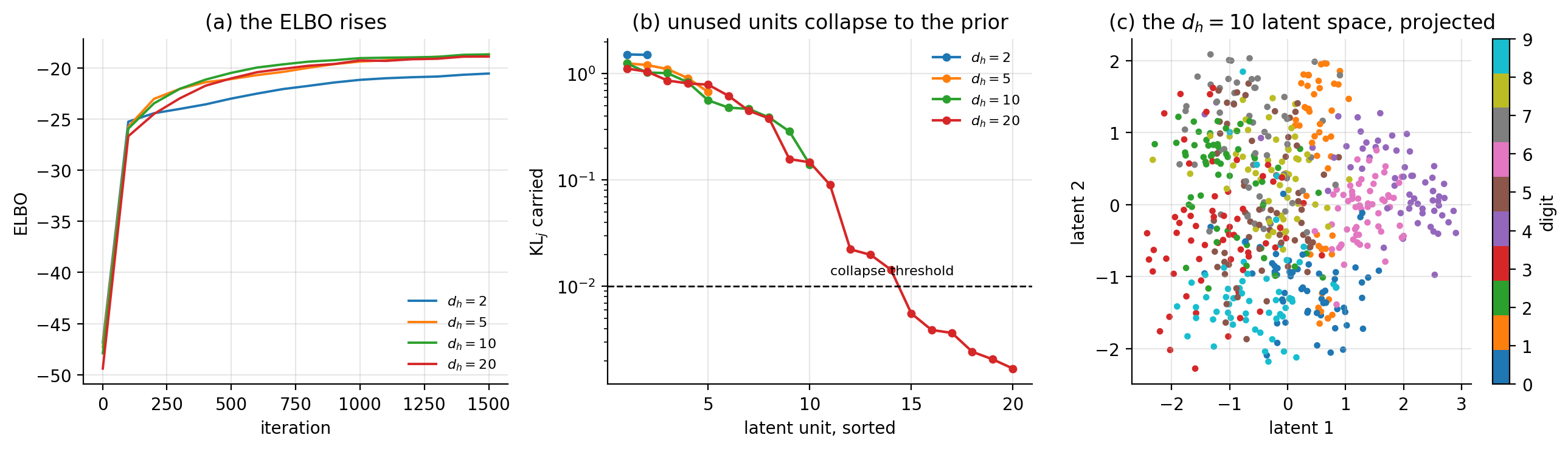
Figure 15.1: (a) The ELBO during training for four latent dimensions; the curves for \(d_h=5,10,20\) are almost on top of one another, which is the first sign that the extra coordinates are not being used. (b) The KL contributed by each latent coordinate, Eq. (15.9), sorted and plotted logarithmically. At \(d_h=20\) the contribution falls below the collapse threshold from the fifteenth coordinate on. (c) The \(d_h=10\) latent means projected onto their two leading principal directions and coloured by digit class: the classes separate, although nothing in Eq. (15.8) asked them to.
Panel (c) is the encouraging counterpart. The model was never shown a label, and the classes nevertheless separate in the latent space. That is the payoff of the prior-matching term: by forcing the codes into a compact, well-covered region it makes the latent space continuous and comparable across inputs, which is exactly what the autoencoder of Chapter 12 failed to do. Recall Figure 12.5(c), where an autoencoder reconstructed a curve beautifully while its code jumped and saturated. The VAE buys a usable latent geometry, and Eq. (15.8) says exactly what it pays: the KL term is the price, measured in nats.
15.6. Implementations in the libraries#
The only unusual element is that the loss depends on intermediate quantities – \(\bm{\mu}\) and \(\log\bm{\sigma}^{2}\) – and not only on the output, so the sampling step must be written explicitly rather than hidden inside a layer. That also makes the comparison against our own implementation unusually clean: Eq. (15.10) turns the randomness into an input, so two implementations given the same weights and the same \(\bm{\epsilon}\) must produce the same number. They do:
=== 1. the ELBO of Eq. (15.objective), identical weights and noise ===
  ELBO, ours   : -15.499610160480
  ELBO, torch  : -15.499610160480
  ELBO, keras  : -15.499610160480
  max |mu_ours - mu_keras|                    : 2.220e-16
  max |KL_ours - KL_torch|, Eq. (15.klclosed) : 2.220e-16

   parameter   shape        |ours - torch|      scale
   enc W1    (20, 16)          6.939e-17   2.639e-01
   enc W2    (16, 8)           1.110e-16   3.528e-01
   dec W1    (4, 16)           1.665e-16   6.378e-01
   dec W2    (16, 20)          8.327e-17   3.969e-01
  worst disagreement: 1.665e-16
That the three agree to twelve decimal places on the value is unremarkable arithmetic. That they agree on the gradient is the point of Section The reparameterisation trick: the estimator is an ordinary differentiable function of the parameters, so three different automatic differentiators applied to three separate implementations return the same thing. A sampling operation would not have had that property, and neither would Eq. (15.12).
import tensorflow as tf
from tensorflow import keras
from tensorflow.keras import layers


class Sampling(layers.Layer):
    """Eq. (15.reparam): h = mu + sigma * eps, with eps an input."""
    def call(self, inputs):
        mu, logvar = inputs
        eps = tf.random.normal(tf.shape(mu))
        return mu + tf.exp(0.5 * logvar) * eps


d, d_h = 784, 16
enc_in = keras.Input(shape=(d,))
e = layers.Dense(256, activation="relu")(enc_in)
mu = layers.Dense(d_h, name="mu")(e)
logvar = layers.Dense(d_h, name="logvar")(e)         # log sigma^2, unconstrained
h = Sampling()([mu, logvar])
encoder = keras.Model(enc_in, [mu, logvar, h], name="encoder")

dec_in = keras.Input(shape=(d_h,))
dd = layers.Dense(256, activation="relu")(dec_in)
logits = layers.Dense(d)(dd)                          # Bernoulli logits
decoder = keras.Model(dec_in, logits, name="decoder")


class VAE(keras.Model):
    def __init__(self, encoder, decoder):
        super().__init__()
        self.encoder, self.decoder = encoder, decoder

    def train_step(self, x):
        with tf.GradientTape() as tape:
            mu, logvar, h = self.encoder(x)
            logits = self.decoder(h)
            rec = -tf.reduce_sum(                     # log p(x|h), Bernoulli
                tf.nn.sigmoid_cross_entropy_with_logits(labels=x, logits=logits),
                axis=1)
            kl = 0.5 * tf.reduce_sum(                 # Eq. (15.klclosed)
                tf.square(mu) + tf.exp(logvar) - logvar - 1.0, axis=1)
            loss = -tf.reduce_mean(rec - kl)          # minimise the negative ELBO
        g = tape.gradient(loss, self.trainable_weights)
        self.optimizer.apply_gradients(zip(g, self.trainable_weights))
        return {"elbo": -loss}


vae = VAE(encoder, decoder)
vae.compile(optimizer=keras.optimizers.Adam(1e-3))
vae.fit(x_train, epochs=30, batch_size=128)
The same in PyTorch, where the reparameterisation is a method:
import torch
import torch.nn as nn
import torch.nn.functional as F


class VAE(nn.Module):
    def __init__(self, d=784, d_h=16, hidden=256):
        super().__init__()
        self.fc = nn.Linear(d, hidden)
        self.fc_mu = nn.Linear(hidden, d_h)
        self.fc_logvar = nn.Linear(hidden, d_h)
        self.dec = nn.Sequential(nn.Linear(d_h, hidden), nn.ReLU(),
                                 nn.Linear(hidden, d))

    def encode(self, x):                              # Eq. (15.encoder)
        e = F.relu(self.fc(x))
        return self.fc_mu(e), self.fc_logvar(e)

    def reparameterise(self, mu, logvar):             # Eq. (15.reparam)
        return mu + torch.exp(0.5 * logvar) * torch.randn_like(mu)

    def forward(self, x):
        mu, logvar = self.encode(x)
        h = self.reparameterise(mu, logvar)
        return self.dec(h), mu, logvar


def negative_elbo(logits, x, mu, logvar):
    """Eq. (15.objective), summed over pixels and averaged over the batch."""
    rec = F.binary_cross_entropy_with_logits(logits, x, reduction="none").sum(1)
    kl = 0.5 * (mu.pow(2) + logvar.exp() - logvar - 1.0).sum(1)
    return (rec + kl).mean()


model = VAE()
opt = torch.optim.Adam(model.parameters(), lr=1e-3)
for epoch in range(30):
    for xb, _ in train_loader:
        xb = torch.bernoulli(xb.view(-1, 784))        # binarise
        logits, mu, logvar = model(xb)
        loss = negative_elbo(logits, xb, mu, logvar)
        opt.zero_grad(set_to_none=True)
        loss.backward()
        opt.step()

# generating new data: draw from the prior and decode, no Markov chain needed
with torch.no_grad():
    samples = torch.sigmoid(model.dec(torch.randn(64, 16)))
The last two lines are worth pausing on. Generation is a single forward pass from a prior sample. Compare Chapter 14, where drawing one sample required running a Markov chain to equilibrium with no way of knowing when it had arrived. That is what the variational construction bought.
15.6.1. The variance that decides the matter#
Section The reparameterisation trick compared the two estimators on a one-dimensional toy problem and Proposition 15.4 predicted that the gap grows with the latent dimension. Measuring it on the actual ELBO, drawing two thousand independent single-sample estimates of the encoder gradient at each \(d_h\) and summing the variance over all encoder parameters:
   d_h   reparam variance   score-function variance   ratio
     1         2.6865e+00                3.5057e+02    130.5
     2         1.3156e+00                1.0648e+03    809.3
     4         1.8912e+00                1.9455e+03   1028.7
     8         2.4841e+00                4.2074e+03   1693.8
    16         1.6908e+00                8.5782e+03   5073.5
    32         1.5594e+00                1.5826e+04  10148.3
Read the two middle columns separately, because they behave completely differently. The reparameterised variance is flat: between \(1.3\) and \(2.7\) across a factor of thirty-two in \(d_h\), with no trend. The score-function variance rises roughly in proportion to \(d_h\), from \(3.5\times10^{2}\) to \(1.6\times10^{4}\). That is exactly the split of Eq. (15.14): the first is governed by the fluctuation of \(\nabla f\), which does not care how many latent dimensions there are, and the second carries an explicit factor \(d_h\) multiplying \(\mathbb{E}[f^{2}]\).
The ratio at \(d_h=32\) is ten thousand. To match the reparameterised estimator’s noise the score-function estimator would need ten thousand times as many samples per step, and a real VAE uses \(d_h\) in the hundreds. Figure 15.2(b) plots both. Even in one dimension the ratio is \(130\) here against the six to eight of Section The reparameterisation trick, and the difference is instructive: there \(f\) was a toy function of order one, here it is a log-likelihood over twenty pixels and therefore of order ten, and Eq. (15.14) makes the score-function variance scale with \(\mathbb{E}[f^{2}]\).
15.6.2. How far is the ELBO from the truth?#
Theorem 15.1 says the ELBO falls short of \(\log p(\bm{x})\) by \(\mathrm{KL}(q_{\bm{\phi}}\|p_{\bm{\theta}}(\bm{h}\mid\bm{x}))\), and every account of variational autoencoders says so. Almost none says how big it is, because the true posterior is unavailable – but Proposition 15.2 provides a way in. Training on the full MNIST set for six epochs and then evaluating \(\mathcal{L}_K\) at increasing \(K\):
=== 2. the ELBO gap, Theorem 15.elbo, measured ===
   d_h      L_1 (ELBO)        L_16        L_128       L_1024    L_1024 - L_1
     2     -155.6954    -153.9240    -153.5464    -153.3117         2.3837
    10     -112.5460    -109.8677    -109.2289    -108.8944         3.6516
    50     -105.7744    -100.9544     -99.6885     -99.0229         6.7515
and in TensorFlow, same architecture and same schedule:
   d_h      L_1 (ELBO)        L_16        L_128       L_1024    L_1024 - L_1
     2     -158.9083    -157.4499    -157.1135    -156.9733         1.9350
    10     -112.8858    -110.3861    -109.7177    -109.4030         3.4828
    50     -105.1233    -100.7442     -99.4499     -98.7592         6.3641
Three things follow, and the third changes how the earlier tables should be read.
The bound behaves as Proposition 15.2 says it must: monotone increasing in \(K\), and flattening – from \(K=128\) to \(K=1024\) the gain is a fraction of a nat, so \(\mathcal{L}_{1024}\) is close to \(\log p\).
The gap is several nats and it grows with the latent dimension: \(2.4\) nats at \(d_h=2\), \(3.7\) at \(d_h=10\), \(6.8\) at \(d_h=50\), with TensorFlow agreeing to within half a nat throughout. A diagonal Gaussian is a worse approximation to the true posterior when there are more coordinates for it to be wrong about, which is Theorem 15.1 made quantitative.
And this reverses a conclusion. On the ELBO, \(d_h=50\) looked no better than \(d_h=20\) and marginally worse than \(d_h=10\) was on the smaller data set of Section Two characteristic failures – the reading offered there was that extra latent capacity is wasted. On \(\mathcal{L}_{1024}\), which is much closer to the quantity we actually care about, \(d_h=50\) is nearly ten nats better than \(d_h=10\): \(-99.0\) against \(-108.9\). The larger model was not worse; its bound was looser, because its posterior is harder to approximate. Comparing models by their ELBOs silently penalises whichever model has the more complicated posterior, and here that penalty was large enough to invert the ranking.
15.6.3. Collapse, and the price of preventing it#
Section Two characteristic failures counted active units against \(d_h\). The other knob is the weight on the KL term – the \(\beta\) of the \(\beta\)-VAE – which controls the collapse directly. On the full MNIST set with \(d_h=50\):
=== 3. posterior collapse against the KL weight beta ===
   beta   test ELBO   active units of 50   mean KL per active
   0.25   -128.8367                  50               1.2817
   0.50   -114.4514                  50               0.8403
   1.00   -110.4756                  50               0.5177
   2.00   -116.6579                  47               0.3350
   4.00   -134.7284                  34               0.2264
The ELBO reported is the true one, at \(\beta=1\), so the table is a comparison of what each \(\beta\) delivers on the objective the model is supposed to optimise. It peaks at \(\beta=1\), which it must – that is the objective being measured – and falls off sharply on both sides. Raising \(\beta\) to \(4\) switches off sixteen of the fifty coordinates and costs twenty-four nats; lowering it to \(0.25\) keeps every coordinate alive and costs eighteen. The mean KL per active unit falls monotonically with \(\beta\) throughout, from \(1.28\) to \(0.23\) nats, which is the compression \(\beta\) is buying: fewer nats through the channel per coordinate. Whether that is worth having depends on what the code is for, and the ELBO cannot tell you – which is the honest summary of the \(\beta\)-VAE literature.
Figure 15.2(c) shows the per-coordinate KL at \(\beta=1\) sorted from largest to smallest. There is no cliff: the values slide smoothly from \(2\) nats down to \(0.02\), and the “number of active units” is an artefact of where the threshold is put. That is worth knowing before quoting one.
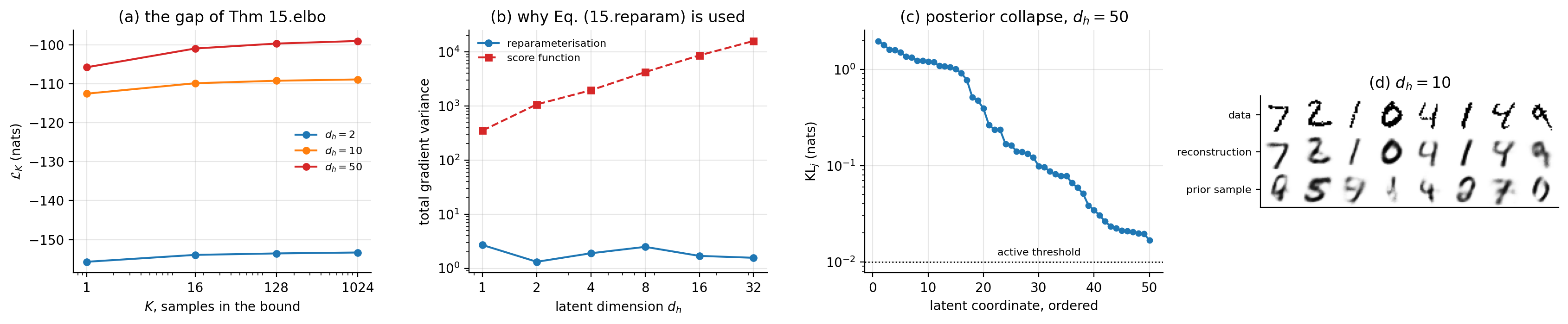
Figure 15.2: (a) The \(K\)-sample bound of Proposition 15.2 against \(K\), for three latent dimensions. \(\mathcal{L}_1\) is the ELBO; \(\mathcal{L}_{1024}\) is close to \(\log p(\bm{x})\), and the vertical distance between them is the gap of Theorem 15.1. (b) The total variance of the two gradient estimators of Section The reparameterisation trick against the latent dimension: the reparameterised one is flat, the score-function one grows linearly, as Eq. (15.14) requires. (c) The average KL contributed by each latent coordinate at \(d_h=50\), sorted; the fall is smooth rather than a cliff. (d) Test digits, their reconstructions and samples decoded from the prior at \(d_h=10\).
15.7. Towards diffusion models#
The natural way to strengthen a VAE is to stop at one latent layer no longer. A hierarchical VAE introduces a chain \(\bm{h}_1,\dots,\bm{h}_T\) of latent variables, and in the Markovian case each depends only on its predecessor:
with \(\bm{h}_0\equiv\bm{x}\). The ELBO of Theorem 15.1 goes through unchanged – the proof used nothing about the dimension or structure of \(\bm{h}\) – and becomes a sum of \(T\) terms, one per level.
Now impose three restrictions on Eq. (15.16), each of which looks like a loss of generality and each of which turns out to buy something:
every latent has the same dimension as the data, so \(\bm{h}_t\in\mathbb{R}^{d}\) and there is no bottleneck at all;
the encoder is not learned but fixed, a prescribed Gaussian that adds a little noise at each step;
the noise schedule is chosen so that \(\bm{h}_T\) is pure \(\mathcal{N}(\bm{0},\bm{I})\), independent of \(\bm{x}\).
What remains is a model with no encoder to train, no bottleneck to collapse, and a prior that matches by construction rather than by paying a KL penalty. The three characteristic difficulties of this chapter have been designed away, and the entire modelling burden falls on the decoder, which must learn to undo one step of noising at a time. That model is a diffusion model, and it is the subject of Chapter 16.
15.8. Summary and the programs#
A variational autoencoder is a latent-variable model whose intractable evidence is replaced by a bound that can be differentiated. Theorem 15.1 is the whole construction: \(\log p(\bm{x})=\mathrm{ELBO}+\mathrm{KL}(q_{\bm{\phi}}\|p(\bm{h}\mid\bm{x}))\), so raising the bound and improving the posterior approximation are one act, and the bound is tight exactly when the encoder recovers the true posterior. We checked the bound directly by quadrature at \(d_h=2\): every gap positive, and varying from \(0.24\) to \(0.65\) nats across data points, which is the mean-field assumption showing its limits.
The ELBO splits into a reconstruction term and a prior-matching term, Eq. (15.8), and the second is what an ordinary autoencoder lacks. It forces the codes towards the prior so that a fresh prior sample decodes to something plausible – generation in one forward pass, with no Markov chain.
The reparameterisation trick, Eq. (15.10), is what made any of it trainable. Both it and the score-function estimator are unbiased; measured on a problem with a known answer, the score-function variance was six to eight times larger in one dimension. Proposition 15.4 says why the gap must grow with the latent dimension – the score-function variance carries an explicit factor \(d_h\) multiplying \(\mathbb{E}[f^{2}]\), the reparameterised one does not – and Section The variance that decides the matter measures it on the real ELBO: the reparameterised variance is flat across a factor of thirty-two in \(d_h\) while the ratio between the two runs from \(130\) to \(10\,148\).
Proposition 15.2 makes the gap of Theorem 15.1 measurable, by squeezing \(\log p\) between \(\mathcal{L}_1=\mathrm{ELBO}\) and the \(K\)-sample bound. On MNIST the gap is \(2.4\) nats at \(d_h=2\) and \(6.8\) at \(d_h=50\): a diagonal Gaussian approximates a harder posterior less well. That measurement changes a conclusion. Ranked by ELBO, \(d_h=50\) looks no better than \(d_h=20\); ranked by \(\mathcal{L}_{1024}\), it is ten nats better than \(d_h=10\). Comparing models by their bounds penalises whichever has the more complicated posterior, and here that was enough to invert the ordering. Both frameworks agree on the whole table to within half a nat.
Two failures are built into the objective rather than accidental. Blurriness follows from a squared-error reconstruction term, which is minimised by the mean of the plausible outputs. Posterior collapse follows from Eq. (15.9), in which each coordinate’s KL is minimised by switching that coordinate off: at \(d_h=20\) only fourteen coordinates survived and the test ELBO was worse than at \(d_h=10\). On the full MNIST set the \(\beta\) sweep of Section Collapse, and the price of preventing it shows the same trade continuously – \(\beta=4\) switches off sixteen of fifty coordinates and costs twenty-four nats – and also shows that the per-coordinate KL falls off smoothly rather than at a cliff, so any count of “active units” is a statement about where the threshold was put. Against all that, the latent space is genuinely usable: the digit classes separated without ever being shown.
The programs are in the directory
doc/BookML/BookPrograms/chapter15_vae.
Every listing above appears there as a numbered file, and three modules run start to finish and reproduce the numbers quoted in the text:
vae.py– the encoder and decoder, the closed-form KL, the reparameterised ELBO and Adam training.verify_vae.py– the KL check against Monte Carlo, the quadrature check that the ELBO bounds the evidence, and the gradient-variance comparison.run_digits.py– the latent-dimension study and the posterior-collapse measurement.cross_check_vae.py– the three-way comparison of Section Implementations in the libraries and the estimator-variance measurement of Section The variance that decides the matter.vae_torch.pyandvae_tf.py– the full-MNIST runs: the latent-dimension sweep, the \(K\)-sample bound of Proposition 15.2 and the \(\beta\) study of Section Collapse, and the price of preventing it.mnist_data.py– a loader that reads MNIST from a local.npz, so that the programs run without network access.
The figure is generated by ch15_figures.py in
doc/BookML/BookFigures; it is not drawn by hand.
15.9. Exercises#
15.9.1. Warm-up exercises#
The bound. (a) Prove Theorem 15.1 by the Jensen route and by the exact route, and say precisely what the second gives that the first does not. (b) Show that the bound is tight if and only if \(q_{\bm{\phi}}(\bm{h}\mid\bm{x})=p_{\bm{\theta}}(\bm{h}\mid\bm{x})\). (c) If \(q\) is restricted to diagonal Gaussians and the true posterior is not one, can the bound ever be tight?
The Gaussian KL. Derive Eq. (15.9) directly, without quoting the general formula, by integrating \(\log q-\log p\) against \(q\). Then show that each term is non-negative and identify the unique minimiser.
Reparameterisation. (a) Verify that Eqs. (15.11) and (15.12) are both unbiased. (b) Compute both variances analytically for \(f(h)=h^{2}\) with \(q=\mathcal{N}(\mu,1)\) and confirm your answer numerically. (c) Explain why Eq. (15.10) cannot be used for a discrete latent variable, and name one thing that can.
Collapse by hand. Consider a VAE whose decoder ignores one latent coordinate entirely. Show from Eq. (15.8) that the ELBO is strictly improved by setting that coordinate’s \(\mu_j=0\) and \(\sigma_j=1\), and compute the improvement in nats.
Blurriness. Let \(p_{\bm{\theta}}(\bm{x}\mid\bm{h})=\mathcal{N}(\bm{f}(\bm{h}),\sigma^{2}\bm{I})\) and suppose a code \(\bm{h}\) is consistent with two data points \(\bm{x}_a\) and \(\bm{x}_b\) occurring equally often. Show that the ELBO is maximised by \(\bm{f}(\bm{h})=(\bm{x}_a+\bm{x}_b)/2\), and comment on what this means for images.
VAE against PCA. Take the decoder linear and the observation noise Gaussian and isotropic. Show that the model becomes probabilistic PCA, Eq. (12.22), and hence by Section The probabilistic view: PPCA that the optimum recovers the principal subspace. What does the KL term correspond to in that limit?
The \(K\)-sample bound. (a) Prove Proposition 15.2, being careful with the random-subset argument that gives monotonicity. (b) Show that \(\mathcal{L}_K\) is the ordinary ELBO of an augmented model with \(K\) latent draws, and identify that model. (c) Explain why \(\mathcal{L}_K-\mathcal{L}_1\) is only a lower bound on the gap of Theorem 15.1, and what would have to be true for it to be the gap exactly.
Estimator variance. (a) Derive Eq. (15.14) and state where the assumption that \(f\) varies slowly compared with \(\|\bm{\epsilon}\|^{2}\) is used. (b) Predict, from the proposition, what happens to the ratio when the decoder output dimension is doubled at fixed \(d_h\). Then measure it. (c) Add a baseline \(b\) to Eq. (15.12), replacing \(f\) by \(f-b\), and find the \(b\) that minimises the variance. How much of the gap does the optimal baseline close?
Measuring the gap. Reproduce Section How far is the ELBO from the truth?. (a) At \(d_h=2\), compare \(\mathcal{L}_{1024}\) against \(\log p(\bm{x})\) computed by two-dimensional quadrature, and check that the bound is where you expect. (b) The gap grows with \(d_h\). Does it grow with the number of active coordinates or with \(d_h\) itself? Design a run that separates the two. (c) Train with the \(K\)-sample bound as the objective rather than as a diagnostic and report what happens to the gap and to the number of active units.
The \(\beta\) trade. (a) Reproduce Section Collapse, and the price of preventing it and add \(\beta=8\) and \(\beta=16\). At what \(\beta\) does the code collapse entirely? (b) Show that at \(\beta\ne1\) the objective is still a valid bound on \(\log p\) for some modified model, and identify it. (c) The chapter reports “active units” at a threshold of \(0.01\) nats. Recompute the counts at \(0.001\) and \(0.1\) and comment on how much of the posterior-collapse literature depends on that choice.
15.9.2. Project-style exercise: a variational autoencoder from scratch#
Part a: the machinery. Implement the encoder, decoder, closed-form KL and reparameterised ELBO. Verify Eq. (15.9) against Monte Carlo, and verify every gradient against finite differences.
Part b: the bound. With \(d_h=1\) or \(2\), compute \(\log p(\bm{x})\) by quadrature and confirm that the ELBO never exceeds it. Then improve the encoder – more capacity, more training, or a full-covariance Gaussian instead of the mean-field one – and show the gap shrinking. Report how much of the gap the mean-field restriction accounts for.
Part c: the estimators. Reproduce the variance comparison of Section The reparameterisation trick, then extend it: plot the variance ratio against latent dimension for \(d_h=1,\dots,50\). Add a baseline to the score-function estimator, as REINFORCE implementations do, and report how much of the gap that closes.
Part d: collapse. Reproduce the latent-dimension study. Then attack the collapse three ways: KL annealing (ramp a weight \(\beta\) on the KL term from \(0\) to \(1\)), a free-bits constraint (do not penalise KL below a floor per coordinate), and a weaker decoder. Report the active-unit count and the test ELBO for each, and say which intervention actually helps and which merely relabels the problem.
Part e: \(\beta\)-VAE. Multiply the KL term of Eq. (15.8) by \(\beta\) and scan \(\beta\in[0,10]\). Plot reconstruction quality and latent-space structure against \(\beta\). At \(\beta=0\) you should recover Chapter 12 exactly – verify that you do – and at large \(\beta\) the model should collapse entirely. Where is the useful regime, and how would you choose \(\beta\) without looking at the answer?
Part f: the latent geometry. Interpolate linearly between the codes of two data points and decode along the path. Do the intermediate images look like data? Repeat with an autoencoder from Chapter 12 trained on the same data and compare. Then quantify it: measure the log-likelihood the model assigns to points along the interpolation.
Part g: towards diffusion. Implement the two-level hierarchical VAE of Eq. (15.16) and derive its ELBO explicitly. Then impose restriction (2) of Section Towards diffusion models – freeze the encoder to a fixed Gaussian that adds noise – and describe what the objective becomes. You will have derived the first step of Chapter 16 yourself.