
5. Chapter 5: Logistic Regression#
Everything so far has predicted a continuous number. We now turn to classification, where the target is a label drawn from a finite set: whether a tumour is malignant or benign, whether a credit card holder will default, which of ten digits a handwritten image shows. The change of target forces a change of model and, more interestingly, a change of loss function – and the new loss will turn out to follow from the same maximum-likelihood argument that produced least squares in Section Deriving least squares from a probability distribution.
Logistic regression is the natural first classifier, and it occupies the same position in this book that linear regression did. It is simple enough that everything can be computed, its cost function is convex so that the optimisation theory of Chapter 4 applies without qualification, and – most importantly for what follows – it is exactly a neural network with no hidden layers. The sigmoid we introduce here is an activation function, the cross-entropy we derive here is the loss used to train classifiers throughout deep learning, and the gradient we compute here reappears as the last step of backpropagation. A reader who understands this chapter thoroughly has already met most of the ingredients of the next one.
5.1. Classification problems#
We consider the case where the responses \(y_i\) are discrete and take values from \(k=0,\dots,K-1\), that is \(K\) classes. The goal is to predict the class from the design matrix \(\bm{X}\in\mathbb{R}^{n\times p}\) of Eq. (1.1), made of \(n\) samples each carrying \(p\) features, and in particular to identify the classes of new, unseen samples.
We specialise for most of the chapter to two classes, with outputs \(y_i=0\) and \(y_i=1\). The outcome might represent whether a credit card holder defaults on their debt,
Why not simply use linear regression?. Before introducing anything new, it is worth seeing why the machinery of Chapter 3 is not adequate. We could fit the linear model
and classify by thresholding, predicting class \(1\) when \(\tilde{y}_i>0.5\) and class \(0\) otherwise. Something like this can be made to work, but it is unsatisfactory for a fundamental reason: the right-hand side of Eq. (5.2) takes values on the entire real axis, while \(y_i\) takes only the values \(0\) and \(1\). A fitted value of \(-3.7\) or \(+2.4\) has no interpretation. Worse, a single distant point drags the fitted line and moves the decision threshold, so that adding a strongly-classified observation can cause a previously correct classification to flip.
One way to force a discrete output is to compose the linear model with a sign function, \(f(s_i)=1\) if \(s_i\ge0\) and \(0\) otherwise. This is the perceptron, historically the first machine learning model and the subject of the opening of the next chapter. It is a hard classifier: each data point is assigned deterministically to a category. In many situations we would rather have a soft classifier, one that outputs the probability of a given category. Probabilities can be thresholded when a decision is needed, but they also express confidence, they can be combined with costs when different errors matter differently, and – as we shall see – they lead to a differentiable cost function, which the step function does not.
An illustration. Data on coronary heart disease (CHD) as a function of age make the point. Plotting whether a person has had CHD (\(y=1\)) or not (\(y=0\)) against age gives two horizontal bands of points, and a straight-line fit through them is visibly meaningless.
import numpy as np
import pandas as pd
import matplotlib.pyplot as plt

chd = pd.read_csv("DataFiles/chddata.csv", names=("ID", "Age", "Agegroup", "CHD"))
plt.scatter(chd["Age"], chd["CHD"], marker="o")
plt.axis([18, 70.0, -0.1, 1.2])
plt.xlabel("Age"); plt.ylabel("CHD")
plt.show()
What is meaningful is the mean value within each age group.
agegroupmean = np.array([0.1, 0.133, 0.250, 0.333, 0.462, 0.625, 0.765, 0.800])
group = np.array([1, 2, 3, 4, 5, 6, 7, 8])
plt.plot(group, agegroupmean, "r-")
plt.axis([0, 9, 0, 1.0])
plt.xlabel("Age group"); plt.ylabel("CHD mean value")
plt.show()
Two features of the resulting curve are decisive. It is confined to the interval \([0,1]\), as any mean of zeros and ones must be. And it is S-shaped: nearly flat at both ends, steepest in the middle. We are looking for a function \(f(y_i\mid x_i)\) giving the expected value of the output for a given input; in linear regression this was \(f(y_i\mid x_i)=\theta_0+\theta_1x_i\), which ranges over the whole real line, whereas here we need \(0\le f(y_i\mid x_i)\le1\) together with the observed S-shape. A function with exactly these properties is the subject of the next section, and we shall interpret it as the probability of observing \(y_i=1\) for a given \(x_i\).
5.2. The logistic function#
The logistic or sigmoid function is
It maps the whole real line onto the open interval \((0,1)\), tends to \(0\) as \(t\to-\infty\) and to \(1\) as \(t\to+\infty\), and takes the value \(\tfrac12\) at the origin. It has the S-shape observed in the CHD group means.
Three properties will be used repeatedly. The first is the reflection identity
immediate from Eq. (5.3), which says that the probability of class \(0\) is obtained from the probability of class \(1\) by flipping the sign of the argument. The second is the derivative,
This is worth deriving once. Writing \(\sigma=(1+e^{-t})^{-1}\),
using \(e^{-t}/(1+e^{-t})=1-\sigma(t)\). Equation (5.5) is remarkable in that the derivative is expressed in terms of the function value alone, with no further exponentials to evaluate. Every gradient in this chapter, and every sigmoid backpropagation step in the next, rests on it. Note also that the derivative is largest at \(t=0\), where it equals \(1/4\), and falls off rapidly in both directions – a fact we shall return to when discussing why deep networks built from sigmoids are hard to train.
The third property is the logit, the inverse function,
the logarithm of the odds. Equation (5.6) is what makes logistic regression linear: we shall model the log-odds as a linear function of the features, even though the probability itself is a non-linear function of them.
Related functions. Two relatives appear later. The step function, \(f(t)=1\) for \(t\ge0\) and \(0\) otherwise, is the hard-classifier limit of the sigmoid and is the perceptron’s activation; it is not differentiable, which is precisely why it cannot be trained by the gradient methods of Chapter 4. The hyperbolic tangent
is a rescaled sigmoid mapping onto \((-1,1)\) rather than \((0,1)\), and is a common activation function in neural networks because its output is centred on zero.
import numpy as np
import matplotlib.pyplot as plt

z = np.arange(-5, 5, 0.1)

fig, ax = plt.subplots(1, 3, figsize=(12, 3.5))
ax[0].plot(z, 1.0 / (1.0 + np.exp(-z)));      ax[0].set_title("sigmoid")
ax[1].plot(z, np.where(z >= 0.0, 1.0, 0.0));  ax[1].set_title("step")
ax[2].plot(z, np.tanh(z));                    ax[2].set_title("tanh")
for a in ax:
    a.grid(True); a.set_xlabel("z")
plt.show()
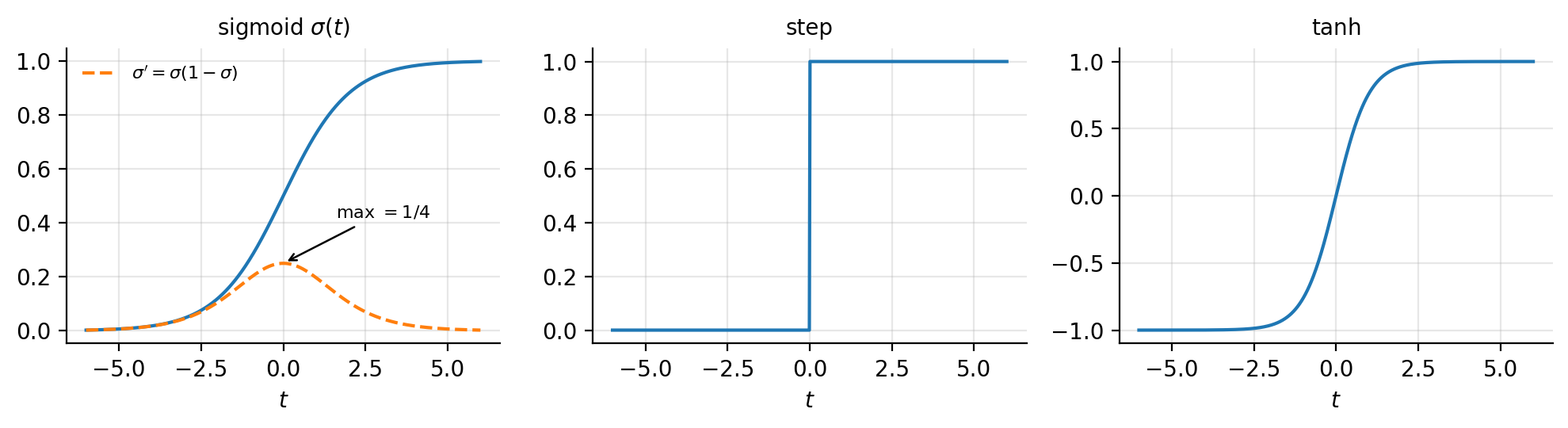
Figure 5.1: The logistic function (5.3) with its derivative \(\sigma'=\sigma(1-\sigma)\), the step function of the perceptron, and \(\tanh\). The derivative attains its maximum of \(1/4\) at the origin and decays rapidly, a fact that returns when deep networks are trained.
5.3. Maximum likelihood and the cross-entropy#
We now derive the cost function. The argument is the one used in Section Deriving least squares from a probability distribution to obtain least squares, with the Gaussian noise model replaced by a Bernoulli one – and the notebox there promised exactly this outcome.
The model. Assume two classes and, to begin with, a single predictor and two parameters. We model the probability of class \(1\) by a sigmoid applied to a linear function of the input,
where \(\bm{\theta}=(\theta_0,\theta_1)\) are the weights we wish to determine. Equation (5.9) is forced: the two probabilities must sum to one. Taking the logit of Eq. (5.8) using Eq. (5.6) gives the equivalent statement
which is the cleanest way to say what logistic regression assumes: the log-odds are linear in the features.
Figure 5.2 shows the consequence in the plane. The decision boundary \(p=\tfrac12\) is a straight line, because it is the locus \(\bm{x}^{T}\bm{\theta}=0\); what is not linear is the probability, which varies smoothly across the boundary at a rate set by \(\|\bm{\theta}\|\). The dashed contours at \(p=0.1\) and \(p=0.9\) mark the region in which the model declines to commit itself, and it is exactly this graded output – rather than the hard assignment of the perceptron – that a soft classifier provides.
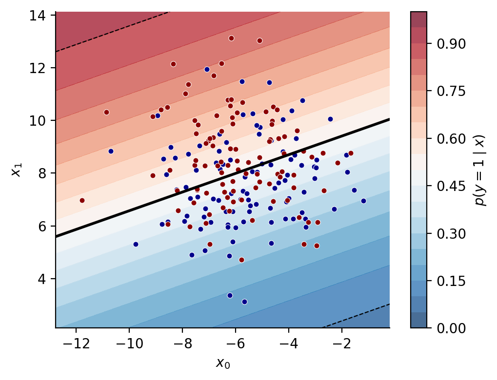
Figure 5.2: Fitted probability \(p(y=1\mid\bm{x})\) for two Gaussian classes. The solid line is the decision boundary \(p=\tfrac12\), a straight line; the dashed contours at \(p=0.1\) and \(0.9\) bound the region of genuine uncertainty.
The likelihood. For a data set \(\mathcal{D}=\{(y_i,x_i)\}\) with binary labels and independent observations, the maximum likelihood principle instructs us to maximise the probability of the data actually seen. A single observation contributes \(p(y_i=1\mid x_i,\bm{\theta})\) if \(y_i=1\) and \(1-p(y_i=1\mid x_i,\bm{\theta})\) if \(y_i=0\); both cases are captured by the single expression \(p^{y_i}(1-p)^{1-y_i}\), in which the exponents switch the factors on and off. Hence
This is a product of Bernoulli probabilities, exactly as Eq. (3.25) was a product of Gaussians.
As in Section Deriving least squares from a probability distribution we take logarithms, both because it turns the product into a sum and because a product of \(n\) numbers smaller than one underflows. The log-likelihood is
The cost function. Since we minimise rather than maximise, the cost is the negative log-likelihood,
This is known in statistics and information theory as the cross entropy, and it is the loss function used to train essentially every classifier in this book.
Substituting Eq. (5.8) and reordering the logarithms gives a form which is both more compact and numerically better behaved. Using \(\log p_i = (\theta_0+\theta_1x_i)-\log[1+\exp(\theta_0+\theta_1x_i)]\) and \(\log(1-p_i)=-\log[1+\exp(\theta_0+\theta_1x_i)]\),
Convexity. The cross entropy is a convex function of \(\bm{\theta}\), so by Section Convexity any local minimiser is a global minimiser. We verify this in Section Gradients, the Hessian and convexity by exhibiting the Hessian and showing it is positive semi-definite. This is a substantial guarantee, and it is why logistic regression is a well-behaved problem in a way that neural networks are not: we may apply any of the methods of Chapter 4 without worrying about which minimum we reach.
Finally, note that just as in linear regression we often supplement the cross entropy with regularisation terms, usually the \(\ell_1\) and \(\ell_2\) penalties of Sections Ridge regression and The Lasso; we return to this in Section More predictors, and regularisation.
Why not squared error?
It is natural to ask why we do not simply minimise \(\sum_i(y_i-p_i)^{2}\), which is also well defined. There are two answers. The statistical one is that the squared error is the maximum-likelihood loss for Gaussian noise, which is the wrong model for a binary outcome; the cross entropy is the correct one for a Bernoulli outcome, exactly as promised in the notebox of Section Deriving least squares from a probability distribution. The practical one is about gradients. Differentiating the squared error brings down a factor \(\sigma'(t)=\sigma(1-\sigma)\) by Eq. (5.5), which is small whenever the prediction is confident, whether or not it is correct. A badly wrong, confidently made prediction therefore produces almost no gradient and the model learns nothing from its worst mistakes. The cross-entropy gradient, as the next section shows, contains no such factor: it is simply the error \(y_i-p_i\). This cancellation is one of the reasons the cross entropy is universal in classification. It is not the only possible loss, however, and Section Other loss functions, and automatic differentiation surveys the alternatives – and fits all of them with a single program.
Figure 5.3 makes the argument visually. The left panel shows the two losses for a point whose true label is \(y=1\): both fall as the prediction improves, and the cross entropy diverges as \(p\to0\) whereas the squared error saturates at one. The right panel shows the gradients, and it is the decisive one. In the shaded region the model is confidently wrong, and there the squared-error gradient has collapsed almost to zero – the model receives no signal from its worst mistakes – while the cross-entropy gradient is at its largest.
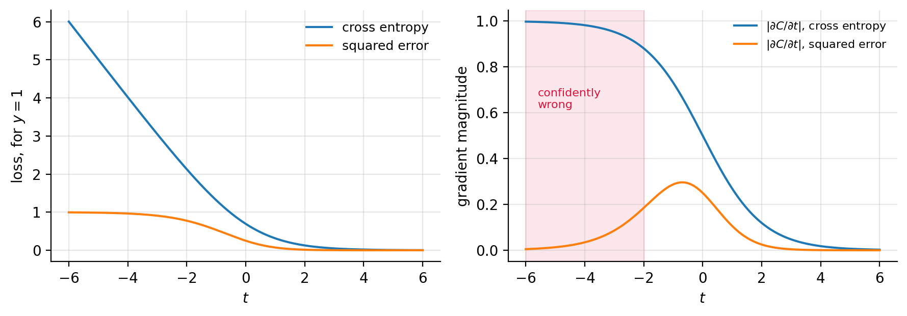
Figure 5.3: Cross entropy and squared error for a single observation with \(y=1\) (left) and the magnitudes of their gradients with respect to \(t=\bm{x}^{T}\bm{\theta}\) (right). In the shaded region the prediction is confidently wrong, and the squared-error gradient vanishes there.
5.4. Gradients, the Hessian and convexity#
Minimising Eq. (5.14) with respect to the two parameters, and using \(\exp(t)/[1+\exp(t)]=\sigma(t)=p_i\), gives
Both have the same structure: the residual \(y_i-p_i\) weighted by the corresponding feature, with the intercept carrying the implicit feature \(1\).
Compact form. Define the vector \(\bm{y}\) of the \(n\) labels, the \(n\times p\) design matrix \(\bm{X}\) containing the inputs including a column of ones, and the vector \(\bm{p}\) of fitted probabilities with entries \(p_i=p(y_i=1\mid\bm{x}_i,\bm{\theta})\). Then Eqs. (5.15) and (5.16) collapse to
This should look extremely familiar. Compare it with the least-squares gradient of Eq. (1.38), \(-\tfrac{2}{n}\bm{X}^{T}(\bm{y}-\bm{X}\bm{\theta})\). The two are identical in form, differing only in that the linear prediction \(\bm{X}\bm{\theta}\) has been replaced by the probability \(\bm{p}=\sigma(\bm{X}\bm{\theta})\) and in an overall constant. In both cases the gradient is the design matrix transposed against the residual, and the algorithmic remark of the notebox in Section The Hessian matrix applies unchanged: the gradient costs two matrix-vector products and never requires a matrix to be formed.
The similarity is not superficial. Both models are generalised linear models: a linear predictor \(\eta_i=\bm{X}_{i,\ast}\bm{\theta}\) is passed through a link function, the identity in one case and the sigmoid in the other, and for the canonical link the maximum-likelihood gradient always takes the form “design matrix transposed times residual”.
The Hessian. Differentiating Eq. (5.17) once more requires the derivative of \(\bm{p}\) with respect to \(\bm{\theta}\), which by Eq. (5.5) and the chain rule (1.50) is \(\partial p_i/\partial\bm{\theta}=p_i(1-p_i)\bm{X}_{i,\ast}\). Defining the diagonal matrix \(\bm{W}\) with entries
we obtain the compact expression
Compare again with least squares, where the Hessian was \(\bm{X}^{T}\bm{X}\) by Eq. (1.44). Logistic regression inserts a diagonal weight matrix between the two factors, and the weights are largest, equal to \(\tfrac14\), where \(p_i=\tfrac12\) – that is for the observations the model is most uncertain about, those nearest the decision boundary. Points far from the boundary have \(p_i\) near \(0\) or \(1\), hence \(W_{ii}\) near zero, and contribute almost nothing to the curvature. The fit is determined by the points near the boundary, which is a first hint of the idea carried to its conclusion by support vector machines.
Convexity, proved. For any vector \(\bm{z}\),
because every \(W_{ii}=p_i(1-p_i)\) is positive for \(0<p_i<1\). The Hessian is therefore positive semi-definite everywhere, so by the second-order condition of Section Convexity the cross entropy is convex and by the result quoted there any stationary point is a global minimum. This is the promised proof.
No closed form. Unlike the normal equations (1.39), setting Eq. (5.17) to zero does not yield a formula for \(\hat{\bm{\theta}}\): the unknown appears inside the non-linear function \(\bm{p}=\sigma(\bm{X}\bm{\theta})\), and no rearrangement extracts it. We must solve numerically, which is why Chapter 4 preceded this one. The situation resembles the Lasso of Section The Lasso – a convex problem without a closed form – although here the obstruction is non-linearity rather than non-differentiability, so ordinary gradient methods apply directly.
5.5. More predictors, and regularisation#
Extending to \(p\) predictors requires no new ideas. The log-odds relation (5.10) becomes
and with \(\bm{x}=[1,x_1,\dots,x_p]\) and \(\bm{\theta}=[\theta_0,\theta_1,\dots,\theta_p]\) the probability is
The gradient (5.17) and Hessian (5.19) are already written in a form valid for any \(p\).
Regularisation. In practice the cross entropy is supplemented with a penalty, exactly as in Chapter 3,
giving the \(\ell_2\) and \(\ell_1\) regularised versions. The gradient of the \(\ell_2\) penalty is \(2\lambda\bm{\theta}\) by Eq. (1.28), so Eq. (5.17) becomes \(-\bm{X}^{T}(\bm{y}-\bm{p})+2\lambda\bm{\theta}\), and the Hessian becomes \(\bm{X}^{T}\bm{W}\bm{X}+2\lambda\bm{I}\), which is positive definite for \(\lambda>0\) and hence strictly convex.
Everything said in Chapter 3 about the two penalties carries over: \(\ell_2\) shrinks coefficients smoothly, \(\ell_1\) sets some exactly to zero and performs variable selection, the intercept should not be penalised, and the features must be standardised first for the penalty to be meaningful. The remarks of Section Scaling, centring and the intercept apply verbatim.
There is one addition specific to classification. If the two classes are
linearly separable – if some hyperplane divides them perfectly – then
the unregularised maximum likelihood problem has no finite solution.
The likelihood can always be increased by scaling \(\bm{\theta}\) up, which
makes every predicted probability more extreme and drives the cost towards
zero without ever attaining it, so \(\|\bm{\theta}\|\to\infty\). Any penalty
\(\lambda>0\) removes the pathology by making the cost eventually increase.
This is one reason scikit-learn regularises by default, with
C playing the role of \(1/\lambda\) – a convention worth remembering
when comparing against one’s own implementation, in the spirit of the
warnings in Section Comparing the three estimators.
Machine learning connection
The conditioning discussion of Section The learning rate and the condition number applies here with a twist. The Hessian is now \(\bm{X}^{T}\bm{W}\bm{X}\), which changes as the fit proceeds because \(\bm{W}\) depends on the current probabilities. Early in training, when all \(p_i\approx\tfrac12\) and \(\bm{W}\approx\tfrac14\bm{I}\), the curvature is essentially \(\tfrac14\bm{X}^{T}\bm{X}\) and the analysis of Chapter 4 carries over directly. As the fit sharpens, the well-classified points drop out of \(\bm{W}\) and the effective Hessian is built from a shrinking subset of the data, typically becoming worse conditioned. A learning rate chosen at the start may therefore be badly wrong later, which is one concrete reason the adaptive methods of Section Why adapt the step size at all – whose \(\bm{v}_t\) tracks a recent average and so follows the changing landscape – are useful even on this convex problem.
5.6. More than two classes: the softmax#
Suppose we wish to extend to \(K\) classes. Taking one class as a reference – conventionally the last – we model each of the remaining \(K-1\) log-odds ratios as linear. With a single predictor for simplicity,
The model is thus specified by \(K-1\) logit transformations. Solving for the probabilities, and using the fact that they must sum to one,
with the reference class taking the remainder,
These sum to one by construction, and setting \(K=2\) recovers Eqs. (5.8) and (5.9), so the binary case is the special case it should be. Extending to more predictors requires only replacing \(\theta_{k0}+\theta_{k1}x_1\) by \(\bm{x}^{T}\bm{\theta}_k\).
The symmetric form. Singling out a reference class is inelegant, and in practice one uses the symmetric parametrisation
which is the softmax function. It is over-parametrised: adding the same vector to every \(\bm{\theta}_k\) leaves all the probabilities unchanged, since the added factor cancels between numerator and denominator, so the parameters are determined only up to a common shift. Fixing \(\bm{\theta}_{K-1}=\bm{0}\) recovers Eq. (5.25), and adding an \(\ell_2\) penalty also removes the redundancy by selecting the smallest representative. The redundancy is harmless in practice and the symmetric form is easier to implement.
The corresponding cost function is the multiclass cross entropy,
where \(y_{ik}\) is the one-hot encoding, equal to one if sample \(i\) belongs to class \(k\) and zero otherwise. For \(K=2\) this reduces to Eq. (5.13). Its gradient with respect to \(\bm{\theta}_k\) retains the familiar structure,
with \(\bm{y}_k\) and \(\bm{p}_k\) the columns of the one-hot targets and of the predicted probabilities for class \(k\) – again design matrix transposed against residual.
A numerical warning. Equation (5.27) must never be evaluated as written. If any \(\bm{x}^{T}\bm{\theta}_k\) is large, \(\exp\) of it overflows. Since the softmax is invariant under subtracting a constant from every score, one subtracts the largest before exponentiating,
which is mathematically identical and numerically safe: every exponent is now non-positive, so no term exceeds one. This trick appears in the implementation of Section An implementation and in every deep learning library.
The softmax will reappear in the next chapter as the output layer of a classification network, where Eq. (5.27) applied to the final linear layer is exactly multinomial logistic regression performed on learned rather than raw features.
5.7. Optimising the cross entropy#
Having no closed form, we must minimise Eq. (5.13) numerically. This is where Chapter 4 is spent, and the good news is that every method there applies without modification: the problem is convex, the gradient is Eq. (5.17), and the Hessian is Eq. (5.19).
Gradient descent. The simplest scheme is Eq. (4.15) with the logistic gradient,
noting the plus sign, which comes from the minus in Eq. (5.17). The stability bound (4.20) applies with \(\lambda_{\max}\) the largest eigenvalue of \(\bm{X}^{T}\bm{W}\bm{X}\); since \(W_{ii}\le\tfrac14\), a safe choice is \(\gamma<8/\lambda_{\max}(\bm{X}^{T}\bm{X})\). For large data sets one uses the minibatch stochastic version of Section Stochastic gradient descent, and in practice one of the adaptive methods of Sections AdaGrad to Adam; Section Stochastic gradient descent for logistic regression runs all of them on a logistic regression with \(50\,000\) observations and measures what each buys.
Newton-Raphson, or iteratively reweighted least squares. Because the Hessian is available in the closed form (5.19), and because \(p\) is often modest, Newton’s method of Section Newton’s method is frequently the method of choice here – one of the few places in this book where it is affordable. Substituting Eqs. (5.17) and (5.19) into the Newton step (4.8),
that is, in matrix form,
with the right-hand side evaluated at the old parameters. Unlike the quadratic case of Eq. (4.9), one step does not suffice, since \(\bm{W}\) and \(\bm{p}\) must be recomputed; but convergence is quadratic and a handful of iterations is typical.
Equation (5.33) has an illuminating rewriting. Defining the adjusted response \(\bm{z}=\bm{X}\bm{\theta}^{\mathrm{old}}+\bm{W}^{-1}(\bm{y}-\bm{p})\), a line of algebra turns it into
which is precisely the weighted least squares solution (3.14) with weights \(\bm{W}\) and targets \(\bm{z}\). Logistic regression is therefore solved by repeatedly performing a weighted linear regression, recomputing the weights at each pass – whence the name iteratively reweighted least squares (IRLS). It is a pleasing connection: the classifier reduces to a sequence of the linear fits of Chapter 3.
In practice one does not form the inverse in Eq. (5.33). Since \(\bm{X}^{T}\bm{W}\bm{X}\) is symmetric positive semi-definite, the step is obtained from a Cholesky factorisation as in Section LU and Cholesky decompositions, or more safely still from the QR or SVD route of Section Ordinary least squares applied to \(\bm{W}^{1/2}\bm{X}\), which avoids squaring the condition number.
import numpy as np

def sigmoid(z):
    """Numerically stable logistic function, Eq. (5.sigmoid)."""
    out = np.empty_like(z, dtype=float)
    pos, neg = z >= 0, z < 0
    out[pos] = 1.0 / (1.0 + np.exp(-z[pos]))
    ez = np.exp(z[neg])                       # avoids overflow for z << 0
    out[neg] = ez / (1.0 + ez)
    return out


def logreg_newton(X, y, n_iter=25, tol=1e-10, ridge=1e-8):
    """Logistic regression by Newton-Raphson, Eq. (5.newton).

    A tiny ridge term keeps X^T W X invertible when the classes are
    separable or W becomes numerically singular.
    """
    n, p = X.shape
    theta = np.zeros(p)
    for it in range(n_iter):
        prob = sigmoid(X @ theta)
        gradient = X.T @ (y - prob)                       # Eq. (5.gradient)
        W = prob * (1.0 - prob)                           # Eq. (5.Wmatrix)
        H = X.T @ (W[:, None] * X) + ridge * np.eye(p)    # Eq. (5.hessian)
        step = np.linalg.solve(H, gradient)               # never invert H
        theta += step
        if np.linalg.norm(step) < tol:
            break
    return theta, it + 1
Note the stable sigmoid. Evaluating \(1/(1+e^{-z})\) directly overflows for large negative \(z\), and the two-branch form above is the standard remedy – the same defensive reasoning as the softmax shift of Eq. (5.30).
Machine learning connection
Which optimiser to use is decided by the
shape of the problem, and logistic regression makes the trade-off unusually
clear. Newton’s method costs \(\bigO(np^{2})\) to form the Hessian and
\(\bigO(p^{3})\) to factorise it, but converges in a handful of iterations; for
\(p\) in the tens or hundreds it is unbeatable, and it is what
scikit-learn uses through its lbfgs and newton-cg
solvers. For \(p\) in the millions – text classification with a bag-of-words
representation, say – the Hessian is unavailable and one falls back on SGD
with an adaptive method. The dividing line is exactly the one drawn in
Section None of these can compete with Newton’s method, and logistic regression sits close enough to
it that both sides are commonly seen.
5.8. An implementation#
We now assemble a class handling both the binary and the multiclass case, trained by gradient descent. It is deliberately written to mirror the equations: the reader should be able to point at each line and name the formula it implements.
import numpy as np

class LogisticRegression:
    """Logistic regression for binary and multiclass classification.

    Binary problems use the sigmoid (5.sigmoid) with the cross entropy
    (5.crossentropy); multiclass problems use the softmax (5.softmax)
    with the multiclass cross entropy (5.multicrossentropy).
    """

    def __init__(self, lr=0.01, epochs=1000, fit_intercept=True, lmbda=0.0):
        self.lr = lr                       # learning rate for gradient descent
        self.epochs = epochs
        self.fit_intercept = fit_intercept
        self.lmbda = lmbda                 # l2 penalty, Eq. (5.penalised)
        self.weights = None
        self.multi_class = False

    @staticmethod
    def _add_intercept(X):
        return np.concatenate((np.ones((X.shape[0], 1)), X), axis=1)

    @staticmethod
    def _sigmoid(z):
        out = np.empty_like(z, dtype=float)
        pos, neg = z >= 0, z < 0
        out[pos] = 1.0 / (1.0 + np.exp(-z[pos]))
        ez = np.exp(z[neg])
        out[neg] = ez / (1.0 + ez)
        return out

    @staticmethod
    def _softmax(Z):
        """Softmax with the shift of Eq. (5.softmaxstable)."""
        expZ = np.exp(Z - np.max(Z, axis=1, keepdims=True))
        return expZ / np.sum(expZ, axis=1, keepdims=True)

    def fit(self, X, y):
        X, y = np.asarray(X, dtype=float), np.asarray(y)
        if self.fit_intercept:
            X = self._add_intercept(X)
        n_samples, n_features = X.shape

        self.classes_ = np.unique(y)
        self.multi_class = len(self.classes_) > 2

        if self.multi_class:
            n_classes = len(self.classes_)
            index = {c: k for k, c in enumerate(self.classes_)}
            Y = np.zeros((n_samples, n_classes))            # one-hot targets
            Y[np.arange(n_samples), [index[c] for c in y]] = 1
            self.weights = np.zeros((n_features, n_classes))

            for _ in range(self.epochs):
                probs = self._softmax(X @ self.weights)
                grad = X.T @ (probs - Y) / n_samples        # Eq. (5.softmaxgradient)
                grad += 2.0 * self.lmbda * self.weights
                self.weights -= self.lr * grad
        else:
            yb = (y == self.classes_[1]).astype(float)      # map labels to {0,1}
            self.weights = np.zeros(n_features)

            for _ in range(self.epochs):
                probs = self._sigmoid(X @ self.weights)
                grad = X.T @ (probs - yb) / n_samples       # Eq. (5.gradient)
                grad += 2.0 * self.lmbda * self.weights
                self.weights -= self.lr * grad
        return self

    def predict_proba(self, X):
        X = np.asarray(X, dtype=float)
        if self.fit_intercept:
            X = self._add_intercept(X)
        if self.multi_class:
            return self._softmax(X @ self.weights)
        p1 = self._sigmoid(X @ self.weights)
        return np.column_stack([1.0 - p1, p1])

    def predict(self, X):
        return self.classes_[np.argmax(self.predict_proba(X), axis=1)]
Note that the gradients carry a factor \(1/n\) absent from Eq. (5.17). This merely rescales the learning rate and is the usual convention, since it makes a sensible \(\gamma\) independent of the size of the data set; but it is one more of the bookkeeping factors that must be matched when comparing implementations.
Synthetic data. To exercise the class we generate Gaussian clusters, one per class.
import numpy as np

def generate_binary_data(n_samples=100, n_features=2, random_state=None):
    """Two Gaussian clusters, class 0 around -2 and class 1 around +2."""
    rng = np.random.default_rng(random_state)
    n0 = n_samples // 2
    n1 = n_samples - n0
    X0 = rng.normal(size=(n0, n_features)) - 2.0
    X1 = rng.normal(size=(n1, n_features)) + 2.0
    return np.vstack((X0, X1)), np.array([0] * n0 + [1] * n1)


def generate_multiclass_data(n_samples=150, n_features=2, n_classes=3,
                             random_state=None):
    """One Gaussian cluster per class, centred on a circle."""
    rng = np.random.default_rng(random_state)
    per = n_samples // n_classes
    Xs, ys = [], []
    for k in range(n_classes):
        angle = 2.0 * np.pi * k / n_classes
        centre = 4.0 * np.array([np.cos(angle), np.sin(angle)])
        centre = np.resize(centre, n_features)
        Xs.append(rng.normal(size=(per, n_features)) + centre)
        ys.append(np.full(per, k))
    return np.vstack(Xs), np.concatenate(ys)


X, y = generate_binary_data(200, random_state=2024)
model = LogisticRegression(lr=0.1, epochs=2000).fit(X, y)
print("binary training accuracy:", np.mean(model.predict(X) == y))

Xm, ym = generate_multiclass_data(300, n_classes=3, random_state=2024)
multi = LogisticRegression(lr=0.1, epochs=2000).fit(Xm, ym)
print("multiclass training accuracy:", np.mean(multi.predict(Xm) == ym))
Both problems are separable by construction, so both accuracies are close to
unity. This is the moment to recall the warning of
Section More predictors, and regularisation: on perfectly separable data the unpenalised
likelihood has no finite maximiser, and the weights grow without bound as
training continues. With a fixed number of epochs the growth is simply
truncated; setting lmbda to a small positive value is the principled
fix.
5.8.1. Logistic regression as a single neuron#
Before we take the class apart with automatic differentiation, it is worth drawing it. Written out for one observation with \(p\) features, the model of Eq. (5.10) is
a weighted sum of the inputs, shifted by the intercept and passed through one non-linear function. Figure 5.4 shows Eq. (5.35) as a diagram: the features enter on the left, each edge carries a parameter, the node \(\Sigma\) forms the linear predictor \(z\), the node \(\sigma\) squashes it into a probability, and, if we also attach the label, the cross entropy of Eq. (5.14) is one more node at the far right. This diagram is the simple perceptron of Rosenblatt, mentioned in Section Classification problems, with one change: the step function that made the perceptron a hard classifier has been replaced by the sigmoid. In the language of Chapter 8, which begins with this very picture, the \(x_j\) are the inputs of an artificial neuron, the \(\theta_j\) are its weights, the intercept \(\theta_0\) is its bias, \(\sigma\) is its activation function and \(z\) its pre-activation. Logistic regression is a neural network with a single neuron and no hidden layer; nothing in this chapter needs to be renamed when we get there.
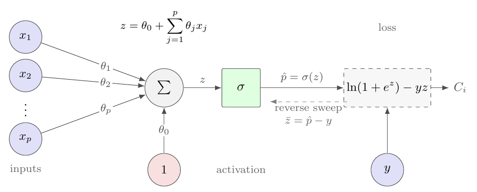
Figure 5.4: Logistic regression drawn as a single artificial neuron, Eq. (5.35): the features \(x_j\) enter on the left, the edges carry the parameters \(\theta_j\), the intercept \(\theta_0\) is the weight of an input permanently fixed at one, the node \(\Sigma\) forms the linear predictor \(z\) and the activation \(\sigma\) turns it into the probability \(\hat p\). Attaching the label \(y\) and the cross entropy of Eq. (5.14) on the right gives the cost of one observation. With the step function in place of \(\sigma\) this is Rosenblatt’s perceptron. Read from right to left, the same diagram is the reverse sweep of Section The same algorithm by automatic differentiation: the sensitivity of the cost to the pre-activation is the residual \(\hat p-y\), and the gradient with respect to \(\theta_j\) is that residual times the input \(x_j\) on the corresponding edge.
The perceptron learning rule. The picture makes the gradient obvious. The cost of one observation depends on the parameters only through \(z\), so by the chain rule \(\partial C_i/\partial\theta_j =(\partial C_i/\partial z)(\partial z/\partial\theta_j)\). The first factor is the derivative of \(\ln(1+e^{z})-y_iz\), namely \(\sigma(z)-y_i=\hat p_i-y_i\), the summand of Eq. (5.15); the second is the input \(x_{ij}\) sitting on the edge of \(\theta_j\) (with \(x_{i0}=1\) for the bias). Hence
and a gradient step on this one observation reads
Equation (5.37) is, up to the choice of activation, Rosenblatt’s original perceptron learning rule of 1958, and with a differentiable activation it is the delta rule of Widrow and Hoff: increase the weight on every input that was active when the output was too small, decrease it when the output was too large, in proportion to the error. Summing Eq. (5.36) over the observations gives back \(\bm{X}^{T}(\bm{p}-\bm{y})\), the gradient (5.17) we derived by algebra in Section Gradients, the Hessian and convexity. Applying Eq. (5.37) one observation, or a few observations, at a time rather than summing first is stochastic gradient descent, to which Section Stochastic gradient descent for logistic regression is devoted.
From the neuron to the computational graph. Figure 5.4 can be read in two ways, and the difference between them is the subject of the next subsection. Read as a model, information flows from left to right: the data \(\bm{x}\) enter, the parameters are fixed numbers on the edges, and a probability comes out. Read as a computational graph in the sense of Section Evaluation traces and the computational graph, it is the same nodes and the same edges, but the roles are exchanged: the parameters are the inputs with respect to which we differentiate, the data are constants of the trace, and the output is the scalar cost \(C_i\). Automatic differentiation in reverse mode is then nothing but the neuron read backwards. The adjoint of the cost is one; it passes through the loss node to give the sensitivity of \(C_i\) to \(\hat p\), through the activation to give the sensitivity to the pre-activation, \(\bar z=\hat p-y\), and from there along each edge to the parameter it carries, picking up the factor \(x_j\) on the way – which is Eq. (5.36) once more, now produced by the fan-out rule rather than by the chain rule written out by hand. The next subsection performs exactly this sweep on the trace of the graph, node by node, and compares it with the forward sweep. The reason for insisting on the picture is what comes after: in Chapter 8 the inputs \(x_j\) of this neuron will themselves be the outputs of other neurons, the reverse sweep will not stop at \(\bar z\) but continue along the edges into the layer before, and Eq. (5.36) will be applied layer by layer. That is backpropagation, and Figure 5.4 is its one-neuron case.
Why the sigmoid, and not the step
The perceptron and logistic regression share Figure 5.4, and the reason the latter replaced the former is visible in it. With the step function as activation the node \(\sigma\) has derivative zero almost everywhere, the reverse sweep dies at that node, and no gradient reaches the parameters: Rosenblatt’s rule had to be justified by a separate convergence argument that works only for separable data. With the sigmoid every node of the graph is differentiable, the sweep passes through, and the rule becomes an instance of gradient descent on a convex cost, with all of Chapter 4 behind it. The same requirement – that the activation be differentiable so that the sweep can pass through it – is what shapes the choice of activation functions in Chapter 8.
5.8.2. The same algorithm by automatic differentiation#
The class of Section An implementation hard-wires the gradient (5.17), which we derived by hand in Section Gradients, the Hessian and convexity and read off the neuron of Figure 5.4 in Section Logistic regression as a single neuron. Logistic regression is simple enough that this was no hardship, but it is also simple enough to show, node by node, what the automatic differentiation of Section Automatic differentiation does with a machine learning cost – and why every framework runs it in reverse mode. We take the compact form (5.14) of the cross entropy and follow one observation \((x_i,y_i)\) through it; the subscript \(i\) is dropped until we reassemble the sum.
The evaluation trace. The inputs of the graph are the parameters, since it is with respect to them that we differentiate; the data \(x\) and \(y\) are constants of the trace. Numbering as in Section Evaluation traces and the computational graph, with \(v_{-1}=\theta_0\) and \(v_0=\theta_1\), a program evaluates the cost of one observation as
so that \(v_2=\theta_0+\theta_1x\) is the linear predictor, \(v_5=\ln(1+e^{v_2})\) the softplus, and \(v_7=\ln(1+e^{z})-yz\) the term in brackets of Eq. (5.14). The computational graph is drawn in Fig. 5.5; it is the neuron of Fig. 5.4 with the parameters as inputs and the loss attached, the summation node split into its elementary operations. Its one structural feature is that the linear predictor \(v_2\) is used twice, by the exponential and by the product with the label, exactly like the fan-out of Section Two examples worked by hand; every generalised linear model has this shape, a linear predictor feeding both the link function and the term that couples it to the label. The local derivatives are
and everything that follows combines these eight numbers.
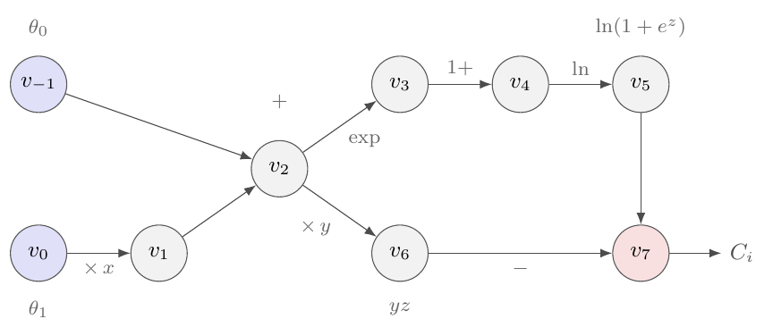
Figure 5.5: The computational graph of the cross entropy of one observation, trace (5.38). The inputs are the two parameters; the data \(x\) and \(y\) enter as constants on the edges. The linear predictor \(z=v_2\) fans out into the softplus branch along the top and the label branch along the bottom, and the reverse sweep of Eq. (5.41) sums the two when it reaches \(v_2\), producing the residual \(p-y\).
Forward mode. A forward sweep, Eq. (4.67), needs a seed. Seeding the first parameter, \((\dot v_{-1},\dot v_0)=(1,0)\), and pushing the tangent through the trace gives
where we recognised \(v_3/v_4=e^{z}/(1+e^{z})=\sigma(z)=p\). The sweep has returned \(\partial C_i/\partial\theta_0=p-y\), which is the summand of Eq. (5.15) – but only that. For \(\partial C_i/\partial\theta_1\) the whole sweep is run again with the seed \((0,1)\): now \(\dot v_1=x\), \(\dot v_2=x\), and every subsequent tangent is the one above multiplied by \(x\), ending in \(\dot v_7=x(p-y)\), the summand of Eq. (5.16). Two parameters, two sweeps. At \(\bm{\theta}=(0.5,0.25)\) for the observation \(x=2\), \(y=1\), the tape holds \(z=1\), \(v_3=2.718\), \(v_4=3.718\), \(v_5=1.313\), \(C_i=0.313\), \(p=0.731\), and the two sweeps return \(-0.269\) and \(-0.538\).
Reverse mode. The reverse sweep, Eq. (4.73), starts from the output with \(\bar v_7=1\) and works back through the trace, using the values on the tape:
One sweep, and both partial derivatives are read off at the input nodes. Two things in Eq. (5.41) deserve a second look. The adjoint of \(v_2\) collects one contribution through each of its successors – the softplus branch contributes \(p\), the label branch contributes \(-y\) – and the sum is the residual \(p-y\): the quantity that Section Gradients, the Hessian and convexity obtained by differentiating the log-odds by hand appears here as the sensitivity of the cost to the linear predictor, produced mechanically by the fan-out rule. And from \(v_2\) down to the parameters the sweep does nothing but multiply the residual by the feature attached to each parameter, \(1\) for the intercept and \(x\) for the slope. Both facts are the derivation of Eqs. (5.15) and (5.16), done by the machine.
The whole data set, and why reverse mode wins. The cost is the sum over observations, \(C=\sum_i C_i\) (or the mean, in the convention of the class above), and its graph is \(n\) copies of Fig. 5.5 hanging from the same parameter nodes and feeding one final summation node. With \(p\) parameters rather than two, \(v_2\) becomes \(z_i=\bm{X}_{i,\ast}\bm{\theta}\) and each observation’s graph has \(p\) input edges instead of two. Consider what the two modes do with it.
In reverse mode the summation node passes \(\bar C_i=1\) to every copy, each copy produces its residual \(r_i=p_i-y_i\) at \(z_i\) by Eq. (5.41), and each parameter node \(\theta_j\) accumulates \(\sum_i X_{ij}\,r_i\) from its \(n\) incoming edges. The sweep has computed
which is Eq. (5.17), in a single pass whose cost is that of the forward evaluation – one matrix–vector product \(\bm{X}\bm{\theta}\) and \(n\) scalar operations – plus one more matrix–vector product \(\bm{X}^{T}\bm{r}\) on the way back: \(\bigO(np)\) in all, a small constant times the cost of evaluating \(C\) itself, precisely as the cheap gradient principle, Proposition 4.2, promises. The tape it needs is the \(n\) values \(z_i\) (from which \(p_i\) follows), a vector.
In forward mode a sweep is seeded with one direction in parameter space. Seeding \(\bm{e}_j\) gives \(\dot z_i=X_{ij}\), then \(\dot C_i=X_{ij}\,r_i\) by the argument that led to Eq. (5.40), and finally \(\dot C=\sum_iX_{ij}r_i\) – one component of the gradient. Each sweep costs \(\bigO(np)\), and there are \(p\) of them: \(\bigO(np^{2})\) for the gradient, a factor \(p\) worse than reverse mode. The disparity is not an artefact of the example. Forward mode propagates one input direction to all outputs; reverse mode propagates one output direction to all inputs. A cost function has one output and \(p\) inputs, and training means asking for all \(p\) sensitivities of that one output. That is the reverse-mode question, and it is why backpropagation – reverse-mode AD on the layered graph of a network – is the algorithm of Chapter 8, where \(p\) runs to millions. The price is the tape: the values of every intermediate node must be kept until the backward sweep has consumed them, which for logistic regression is \(n\) numbers and for a deep network is every activation of every layer. Forward mode keeps nothing but the current tangent, and remains the right tool when the inputs are few and the outputs many – the Jacobian of a network’s outputs with respect to one or two physical parameters, or the derivatives with respect to the spatial coordinates in Chapter 9.
The listing below runs both sweeps, first on the single observation of
Fig. 5.5 – the reverse sweep written out by hand as
in Eq. (5.41), and both modes obtained from JAX with
jax.jvp and jax.grad – and then on a data set, where the
reverse-mode gradient is checked against Eq. (5.17) and the
two modes are timed against the cost of evaluating \(C\) alone. The
functions are written as ordinary NumPy-style code; JAX derives the trace
from them.
import time
import numpy as np
import jax
jax.config.update("jax_enable_x64", True)
import jax.numpy as jnp

def cross_entropy_one(theta0, theta1, x, y):
    """The trace of Eq. (5.adtrace) for one observation, one line per node."""
    v1 = theta1 * x
    v2 = v1 + theta0
    v3 = jnp.exp(v2)
    v4 = 1.0 + v3
    v5 = jnp.log(v4)
    v6 = y * v2
    return v5 - v6

def reverse_sweep(theta0, theta1, x, y):
    """Eq. (5.adreverse) by hand: forward evaluation onto the tape, then back."""
    v1 = theta1 * x; v2 = v1 + theta0; v3 = np.exp(v2); v4 = 1.0 + v3   # tape
    b7 = 1.0
    b5, b6 = b7, -b7
    b4 = b5 / v4
    b3 = b4
    b2 = b3 * v3 + b6 * y                  # fan-out: two successors, one sum
    b1 = b2
    return float(b2), float(b1 * x)        # dC/dtheta0, dC/dtheta1

x, y = 2.0, 1.0
theta = jnp.array([0.5, 0.25])
cost_one = lambda th: cross_entropy_one(th[0], th[1], x, y)
print("C_i =", float(cost_one(theta)))
for k in range(2):                         # forward mode: one sweep per parameter
    _, tangent = jax.jvp(cost_one, (theta,), (jnp.eye(2)[k],))
    print(f"forward sweep, seed e_{k}: dC/dtheta_{k} = {float(tangent):.6f}")
print("reverse sweep, jax.grad:", np.asarray(jax.grad(cost_one)(theta)))
print("reverse sweep, by hand: ", reverse_sweep(0.5, 0.25, x, y))

# the whole data set: mean cross entropy, Eq. (5.crossentropycompact) / n
def cost(theta, X, y):
    z = X @ theta
    return jnp.mean(jnp.logaddexp(0.0, z) - y * z)

rng = np.random.default_rng(2024)
n = 5000
for p in (20, 200, 1000):
    X = jnp.asarray(np.column_stack([np.ones(n), rng.normal(size=(n, p - 1))]))
    yb = jnp.asarray(rng.integers(0, 2, n).astype(float))
    th = jnp.zeros(p)
    value = jax.jit(cost)
    reverse = jax.jit(jax.grad(cost))          # one reverse sweep
    forward = jax.jit(jax.jacfwd(cost))        # p forward sweeps
    for fn in (value, reverse, forward):       # compile before timing
        fn(th, X, yb).block_until_ready()
    p_hat = jax.nn.sigmoid(X @ th)
    g_hand = X.T @ (p_hat - yb) / n            # Eq. (5.gradient) / n
    print(f"p = {p:4d}: max|reverse - hand| = "
          f"{float(jnp.max(jnp.abs(reverse(th, X, yb) - g_hand))):.1e}", end="")
    for name, fn in (("value", value), ("reverse", reverse), ("forward", forward)):
        t0 = time.perf_counter()
        for _ in range(10):
            fn(th, X, yb).block_until_ready()
        print(f"   {name} {1e3 * (time.perf_counter() - t0) / 10:7.2f} ms", end="")
    print()
C_i = 0.3132616875182228
forward sweep, seed e_0: dC/dtheta_0 = -0.268941
forward sweep, seed e_1: dC/dtheta_1 = -0.537883
reverse sweep, jax.grad: [-0.26894142 -0.53788284]
reverse sweep, by hand:  (-0.2689414213699952, -0.5378828427399904)
p =   20: max|reverse - hand| = 3.5e-17   value    0.13 ms   reverse    0.19 ms   forward    0.41 ms
p =  200: max|reverse - hand| = 6.8e-17   value    0.32 ms   reverse    0.47 ms   forward    4.53 ms
p = 1000: max|reverse - hand| = 9.7e-17   value    1.59 ms   reverse    3.31 ms   forward   85.92 ms
The single-observation numbers are those quoted above, and the hand-written
sweep, the forward sweeps and jax.grad agree to rounding. On the
data set the reverse-mode gradient matches Eq. (5.17) to
\(10^{-16}\), and the timings (from a laptop, and only their ratios matter)
say the rest: the reverse-mode gradient costs between \(1.4\) and \(2\) times
the evaluation of \(C\) whatever the number of parameters, as
Proposition 4.2 requires, while the forward-mode
gradient costs \(3\), \(14\) and \(54\) evaluations for \(p=20\), \(200\) and \(1000\),
growing with \(p\) as predicted – less steeply than the factor \(p\) itself
because JAX vectorises the \(p\) sweeps into one matrix product, but without
bound. Section One program for every loss takes the consequence: with the
gradient supplied by one reverse sweep the loss can be changed at will,
and no derivative need ever be written down again.
Machine learning connection
The residual \(p_i-y_i\) that the reverse sweep produces at the linear predictor is the object that every training loop in this book propagates. In a neural network the linear predictor of the last layer is followed by more layers of the same kind, and the reverse sweep continues through them: the adjoint of each layer’s output is multiplied by the transposed weight matrix and by the derivative of the activation, layer by layer, until it reaches the first weights. That is backpropagation, Chapter 8, and Eq. (5.41) is its one-layer special case.
5.9. Stochastic gradient descent for logistic regression#
The two optimisers of Section Optimising the cross entropy – gradient descent and Newton’s method – both touch every observation before they move the parameters once. For the few hundred points of the examples so far this is of no consequence. It becomes the whole story when \(n\) is large, and Section Stochastic gradient descent argued in general terms that the remedy is to update on minibatches: for a cost that is a sum over observations the minibatch gradient is an unbiased estimate of the full one at a fraction of the price, and the statistical accuracy worth having is reached after a few passes over the data. The cross entropy is such a sum, and logistic regression is the simplest model on which the argument can be checked rather than merely asserted. We do so here, and then run the adaptive methods of Chapter 4 on the same problem, so that when the same loop reappears in Chapter 8 with a network in place of the neuron, nothing about the optimiser will be new.
5.9.1. Minibatches and the per-observation gradient#
In the \(1/n\) convention of the class of Section An implementation the cost is the mean of the per-observation costs of Eq. (5.14),
and each term has the gradient (5.36), \(\nabla c_i=(p_i-y_i)\bm{x}_i\), which we read off the neuron of Figure 5.4. A minibatch \(B\) of \(M\) observations drawn without replacement gives the estimate
where \(\bm{X}_B\) holds the \(M\) selected rows of the design matrix. This is Eq. (5.17) restricted to the rows in \(B\) and divided by \(M\), so the code that computes it is the code that computes the full gradient, handed fewer rows. By Eq. (4.37) it is unbiased, \(\mathbb{E}[\bm{g}_B]=\nabla C\), with a variance that scales as \(1/M\); the update
is Eq. (4.36) for the cross entropy, and with \(M=1\) it is the delta rule (5.37) applied to one observation at a time. One pass over the data, an epoch, consists of \(n/M\) such updates, against a single update of gradient descent.
What an epoch costs, and what it buys. The count of Eq. (4.38) transfers directly: the minibatch gradient (5.44) is one matrix–vector product \(\bm{X}_B\bm{\theta}\), \(M\) evaluations of the sigmoid and one product \(\bm{X}_B^{T}\bm{r}_B\), about \(4Mp\) floating-point operations, so that an epoch of SGD costs the same \(4np\) as one step of gradient descent. The question is therefore how much each of the two buys per pass over the data, and the two extremes are easy to state. Gradient descent descends at the rate set by the condition number of the Hessian, Eq. (4.26), and needs of order \(\kappa\ln(1/\epsilon)\) passes to reach an excess cost \(\epsilon\). Stochastic gradient descent makes \(n/M\) moves per pass; early on, when the parameters are far from the optimum, almost every one of them points downhill and the method covers in one epoch what gradient descent covers in hundreds. Late in the run the minibatch noise takes over: at a constant learning rate the iterate does not settle at the minimum but equilibrates in the cloud of Eq. (4.41), of excess cost proportional to \(\gamma/M\), and only a decaying learning rate removes it. The relevant accuracy is set by statistics, as in Section Stochastic gradient descent. The minimiser \(\hat{\bm{\theta}}\) of the empirical cross entropy is the maximum-likelihood estimate of Section Deriving least squares from a probability distribution, and the classical result on the likelihood ratio says that \(2n\,[C(\bm{\theta}_{\mathrm{true}})-C(\hat{\bm{\theta}})]\) is asymptotically \(\chi^{2}\)-distributed with \(p\) degrees of freedom, so the parameters that generated the data sit at an excess cost of about \(p/(2n)\) above the empirical minimum. Optimising below that level chases the noise of this particular sample; it is the analogue for the cross entropy of the floor \(\sigma^{2}p/n\) of Eq. (4.39).
The learning rate of gradient descent. For the comparison to be fair, gradient descent must be given its best constant learning rate, and logistic regression has a feature here that least squares does not. The Hessian \(\bm{X}^{T}\bm{W}\bm{X}/n\) of Eq. (5.19) changes along the path, because the weights \(W_{ii}=p_i(1-p_i)\) do. At the starting point \(\bm{\theta}=\bm{0}\) every \(p_i\) equals \(\tfrac12\), every weight equals its maximum \(\tfrac14\), and the stability bound (4.20) reads
the safe choice already quoted in Section Optimising the cross entropy. As the fit sharpens the weights shrink, the Hessian becomes smaller, and a larger step would be admissible near the optimum – but a step chosen for the optimum overshoots at the start, where the curvature is largest. A constant learning rate must respect the largest curvature met along the way, and Eq. (5.46) is it.
5.9.2. Gradient descent against SGD, measured#
We construct a problem large enough for the difference to show and small enough to run in seconds: \(n=50\,000\) observations and \(p=20\) parameters, an intercept and nineteen standardised features with the same autoregressive correlation of \(0.9\) between neighbouring columns as in Section Stochastic gradient descent, so that the design is strongly correlated. The labels are drawn as \(y_i\sim\mathrm{Bernoulli}(\sigma(\bm{x}_i^{T} \bm{\theta}_{\mathrm{true}}))\) from a known parameter vector; \(40\%\) of them are ones, and even the true parameters classify only \(76.7\%\) of the points correctly, because the classes overlap. Newton’s method of Section Optimising the cross entropy converges in seven iterations to the reference value \(C(\hat{\bm{\theta}})=0.47624\), against which every excess cost below is measured; the Hessian there has condition number \(\kappa=173\), and \(\lambda_{\max}(\bm{X}^{T}\bm{X}/n)=10.9\) gives the learning rate \(\gamma=0.73\) of Eq. (5.46) for gradient descent. The excess cost of \(\bm{\theta}_{\mathrm{true}}\) is \(2.7\times10^{-4}\), close to the \(p/(2n)=2\times10^{-4}\) of the \(\chi^{2}\) argument; this is the dotted line in Figure 5.6, and the level below which further optimisation is pointless.
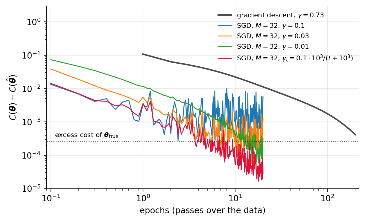
Figure 5.6: Excess cross entropy \(C(\bm{\theta})-C(\hat{\bm{\theta}})\) against passes over the data for the logistic regression problem of Section Gradient descent against SGD, measured (\(n=50\,000\), \(p=20\), \(\kappa=173\)). Gradient descent uses the learning rate (5.46); the SGD runs use minibatches of \(M=32\), the cost being recorded ten times per epoch, at three constant learning rates and with the decaying schedule \(\gamma_t=0.1\cdot10^{3}/(t+10^{3})\). The dotted line is the excess cost of the parameters that generated the data, about \(p/(2n)\). After a single epoch every SGD run is where gradient descent is after twenty. The constant-rate runs then equilibrate in a cloud whose size grows with \(\gamma\), as Eq. (4.41) predicts, the smallest rate reaching within twenty epochs the level gradient descent needs two hundred for; only the decaying schedule continues downwards.
Figure 5.6 and the first block of the output below tell the same story. Gradient descent reduces the excess cost to \(1.1\times10^{-1}\) after one pass, \(3.9\times10^{-2}\) after five, \(1.1\times10^{-2}\) after twenty and reaches \(4.1\times10^{-4}\), about the statistical floor, only after \(200\) passes; the slow, steady slope is the rate \((1-2/\kappa)^{k}\) of a problem with \(\kappa=173\). Stochastic gradient descent with \(M=32\) and \(\gamma=0.01\) is at \(1.8\times10^{-3}\) after five passes and \(3.2\times10^{-4}\) after twenty, so that five epochs of SGD are worth about a hundred of gradient descent and twenty are worth two hundred. Since an epoch of either costs the same \(4np\) operations, this is a factor of ten to twenty in computation, obtained without tuning anything. With the decaying schedule the excess is \(3.0\times10^{-4}\) after five epochs and \(2.8\times10^{-5}\) after twenty – an order of magnitude below the floor, and still falling. The larger constant rates show the other side of the coin: \(\gamma=0.1\) is fastest in the first epoch but then oscillates in a band an order of magnitude wide, and the band for \(\gamma=0.03\) is narrower by about the ratio of the learning rates, as Eq. (4.41) says it should be. One more column of the output deserves attention: the accuracy. Gradient descent classifies \(68.8\%\) of the training points correctly after one pass, \(74.3\%\) after five and \(76.1\%\) after twenty, while both SGD runs of the listing are at \(76.7\%\) after twenty epochs, the accuracy of the true parameters. The accuracy saturates long before the cost does – an excess cost of \(10^{-3}\) already gives an accuracy within half a percent of the best possible – which is why, for classification, a few epochs of SGD are usually all that is ever run.
5.9.3. AdaGrad, RMSProp and Adam on the same problem#
The three adaptive methods of Sections AdaGrad to Adam replace the single learning rate of Eq. (5.45) by one per parameter, obtained from a running average of the squared minibatch gradients: AdaGrad accumulates the squares, Eq. (4.47), RMSProp averages them with exponential forgetting, Eq. (4.50), and Adam adds a momentum-like average of the gradient itself with bias corrections, Eq. (4.57). All three are the diagonally preconditioned iteration of Eq. (4.43), and Chapter 4 drew two conclusions from that form: the preconditioner equalises the curvature along the coordinate axes and therefore undoes any difference in the scales of the features, but it can do nothing about curvature caused by correlation between them, which is not diagonal. Logistic regression lets us test both conclusions with one switch, because the data of the previous subsection come standardised, and we may unstandardise them.
Figure 5.7 shows the four stochastic methods – plain SGD and the three adaptive ones, minibatches of \(32\) throughout – and gradient descent, first on the standardised features of Figure 5.6 and then on the same data with each feature column multiplied by a fixed random factor between \(0.1\) and \(10\), the kind of disparity in units that raw data carry. For each method the constant learning rate was chosen from a grid of five values a factor of \(\sqrt{10}\) apart as the one with the smallest mean excess cost over epochs \(15\) to \(20\); the listing below runs the winners, and Table 5.1 collects the numbers.
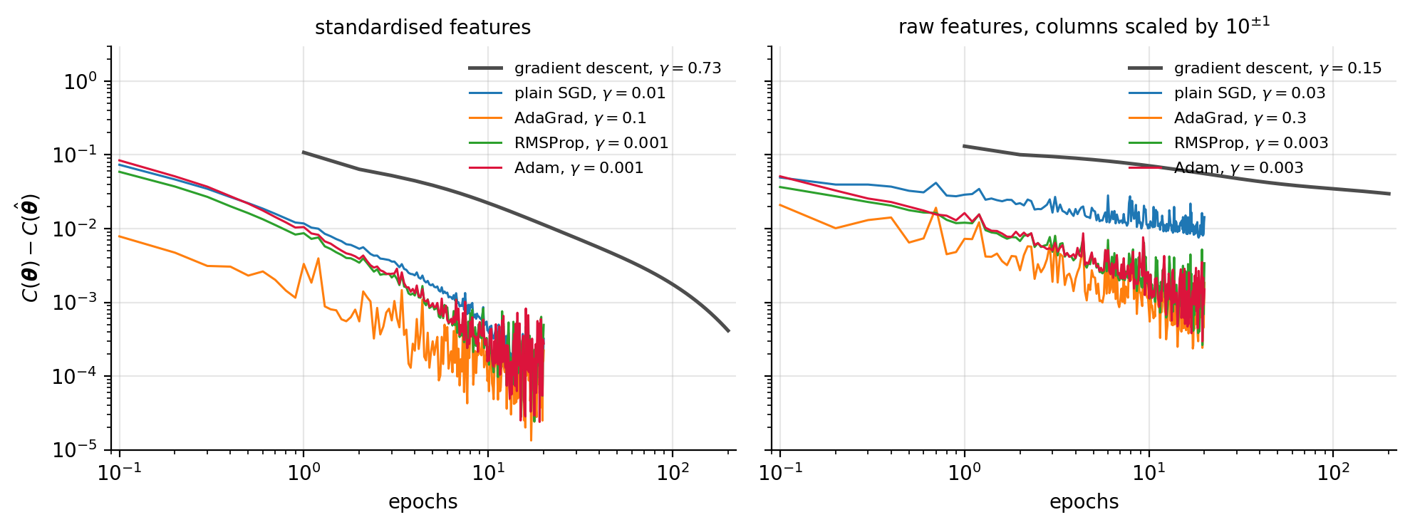
Figure 5.7: Plain SGD, AdaGrad, RMSProp and Adam, all with \(M=32\) and each at the best of five constant learning rates, against gradient descent at the learning rate (5.46), on the logistic regression problem of Section Gradient descent against SGD, measured. Left: standardised features, \(\kappa=173\). Right: the same data with each feature column multiplied by a random factor between \(0.1\) and \(10\), which raises the condition number of the Hessian at the optimum to \(4.4\times10^{4}\) and the excess cost of the two plain-gradient methods by nearly two orders of magnitude, while the three adaptive methods lose less than one. On standardised features the four stochastic methods are indistinguishable after ten epochs.
Method |
\(\gamma\) |
excess, 5 epochs |
mean, 15–20 |
accuracy |
|---|---|---|---|---|
standardised features, \(\kappa=173\) |
||||
gradient descent (200 epochs) |
\(0.73\) |
\(3.9\times10^{-2}\) |
\(4.1\times10^{-4}\) |
\(0.7671\) |
SGD |
\(0.01\) |
\(1.8\times10^{-3}\) |
\(1.9\times10^{-4}\) |
\(0.7666\) |
SGD, \(\gamma_t=0.1\cdot10^{3}/(t+10^{3})\) |
\(0.1\) |
\(3.0\times10^{-4}\) |
\(5.1\times10^{-5}\) |
\(0.7671\) |
AdaGrad |
\(0.1\) |
\(3.0\times10^{-4}\) |
\(1.3\times10^{-4}\) |
\(0.7670\) |
RMSProp |
\(0.001\) |
\(9.4\times10^{-4}\) |
\(2.3\times10^{-4}\) |
\(0.7663\) |
Adam |
\(0.001\) |
\(9.7\times10^{-4}\) |
\(2.2\times10^{-4}\) |
\(0.7666\) |
raw features, \(\kappa=4.4\times10^{4}\) |
||||
gradient descent (200 epochs) |
\(0.15\) |
\(8.6\times10^{-2}\) |
\(3.0\times10^{-2}\) |
\(0.7471\) |
SGD |
\(0.03\) |
\(1.8\times10^{-2}\) |
\(1.2\times10^{-2}\) |
\(0.7585\) |
AdaGrad |
\(0.3\) |
\(2.2\times10^{-3}\) |
\(9.4\times10^{-4}\) |
\(0.7657\) |
RMSProp |
\(0.003\) |
\(3.6\times10^{-3}\) |
\(1.7\times10^{-3}\) |
\(0.7647\) |
Adam |
\(0.003\) |
\(3.3\times10^{-3}\) |
\(1.3\times10^{-3}\) |
\(0.7656\) |
Table 5.1: Excess cross entropy \(C(\bm{\theta})-C(\hat{\bm{\theta}})\) and training accuracy for the methods of Figure 5.7, from the output of the listing below. Gradient descent is listed after \(200\) epochs, the stochastic methods after \(20\); the column “mean” averages the excess cost at the ends of epochs \(15\) to \(20\), which smooths the fluctuations of the constant-rate runs. The excess cost of the parameters that generated the data is \(2.7\times10^{-4}\) in both cases.
Three things stand out. First, on standardised features the adaptive methods bring nothing that plain SGD does not already have: after ten epochs all four sit at the statistical floor, within a factor of two of one another, and the ordering among them changes from epoch to epoch with the noise. The condition number \(\kappa=173\) of this problem comes from the correlation between the columns, not from their scales, and a diagonal preconditioner cannot see it. Second, on the raw features the picture changes completely. Gradient descent, forced by Eq. (5.46) to a learning rate five times smaller, is at an excess cost of \(3\times10^{-2}\) after \(200\) epochs, worse than SGD on the standardised data was after one; plain SGD is at \(10^{-2}\) after twenty epochs, with a training accuracy nearly a full percent below the optimum, and no constant learning rate does better, since the step that suits the columns scaled by \(10\) crawls on those scaled by \(0.1\) and the reverse diverges. The three adaptive methods recover an order of magnitude of that loss, ending at \(10^{-3}\) with accuracies within a quarter of a percent of the optimum, because their per-parameter learning rates absorb the column scales, as the scale invariance of Section Why adapt the step size at all says they must. They do not recover it all: a factor of five to ten remains against the standardised case, and we return to where it comes from below. Third, the learning rates that work differ by two orders of magnitude between the methods, and this is not a matter of tuning but of units: for plain SGD \(\gamma\) multiplies a gradient, while for RMSProp and Adam the update \(\gamma\,\bm{g}/\sqrt{\bm{v}}\) has the size of \(\gamma\) itself in every coordinate (Section Adam), so \(\gamma\) is a step length in parameter space and \(10^{-3}\) is a sensible value; AdaGrad’s ever-growing accumulator shrinks its steps as \(1/\sqrt{t}\), Eq. (4.48), which is why it tolerates, and needs, a rate a hundred times larger.
What the adaptive methods remove, and what they do not.
It is tempting to blame the correlation for the factor of five to ten that the adaptive methods still lose on the raw features, but the correlation is just as present in the standardised data, where all of them reach the floor. The explanation lies elsewhere, and it is worth making precise, because it shows what a per-parameter learning rate can and cannot do. The raw features are the standardised ones in other units, \(x'_j=s_jx_j\), and since the model is the same,
The curvature is where the condition number \(4.4\times10^{4}\) comes from, and a diagonal preconditioner removes the scales from it exactly: with \(\bm{D}=\mathrm{diag}(\bm{H}')\) every \(s_j\) cancels in \(\bm{D}^{-1/2}\bm{H}'\bm{D}^{-1/2}\), and the condition number of that matrix is \(189\) for the raw and for the standardised data alike. This is what rescues the adaptive methods where plain SGD, with a single \(\gamma\) dictated by the largest column, fails. It is also why they gain nothing on standardised features: \(189\) is no better than the \(173\) we started from, because what is left is the correlation, which sits off the diagonal.
What Eq. (5.47) does not leave invariant is the distance each parameter has to travel. The update of Adam and RMSProp has a length of about \(\gamma\) in every coordinate, whatever its unit, Eq. (4.58); but the parameters now live on very different scales, from \(\hat\theta'_j=7.2\) for the column with the smallest factor, \(s_j=0.10\), to \(\hat\theta'_j=0.08\) for the one with the largest, \(s_j=6.2\). Measured in the standardised units, in which all parameters are of order one, a step is \(\gamma s_j\): sixty times longer for the largest column than for the smallest. Figure 5.8 follows Adam for sixty epochs on both versions of the data and shows the two consequences. The parameters of the small columns arrive late: the largest of them is \(87\%\), \(54\%\), \(32\%\), \(13\%\) and \(2\%\) short of its optimum after \(1\), \(5\), \(10\), \(20\) and \(40\) epochs, so that at the twenty epochs of Table 5.1 the run has simply not finished. The parameters of the large columns rattle: for them \(\gamma=0.003\) is a step eighteen times that of the standardised run, and over epochs \(50\) to \(60\) their root-mean-square error is \(0.05\), against \(0.002\) for the small columns and \(0.007\) for every parameter of the standardised run. No single \(\gamma\) is right for both groups. A smaller one, \(\gamma=0.001\), quiets the rattle but makes the late parameters three times later: the excess cost is \(2.1\times10^{-3}\) after twenty epochs and reaches \(2.5\times10^{-4}\) only after sixty. A larger one, \(\gamma=0.01\), brings every parameter in within five epochs and then rattles at \(4\times10^{-3}\) for as long as we care to run. A decaying schedule would reconcile the two, at the price of two more constants to tune; on the standardised features none of this is needed. The adaptive methods equalise the step, not the distance to go; standardising the features equalises both, and that is why it helps every method in Table 5.1, including the ones that are invariant to the scale of the gradient.
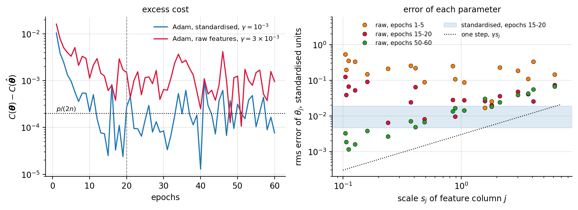
Figure 5.8: Adam with \(M=32\) followed for sixty epochs on the standardised features (\(\gamma=10^{-3}\)) and on the raw ones (\(\gamma=3\times10^{-3}\)), the learning rates of Table 5.1. Left: excess cost at the end of each epoch; the dashed line marks the twenty epochs of the table, the dotted line the floor \(p/(2n)\). Right: root-mean-square error of each parameter of the raw run, converted to standardised units, against the scale \(s_j\) of its column, over three windows of epochs; the band is the range of the standardised run and the dotted line the length \(\gamma s_j\) of one step in these units, Eq. (5.47). The parameters of the small columns arrive late, those of the large columns never stop rattling.
The listing runs every method of Table 5.1. The optimiser is the step function of Section Implementations; the data loop knows nothing about which method it is driving, and the gradient function is the same for a minibatch as for the full data, which is all that Eq. (5.44) requires.
import numpy as np

def sigmoid(t):                          # the stable form of Section 5.7
    a = np.exp(-np.abs(t))
    return np.where(t >= 0, 1.0 / (1.0 + a), a / (1.0 + a))

def make_data(n=50_000, p=20, rho=0.9, seed=2026):
    """AR(1)-correlated standardised features, Bernoulli labels."""
    rng = np.random.default_rng(seed)
    z = rng.normal(size=(n, p - 1))
    xc = np.empty_like(z); xc[:, 0] = z[:, 0]
    for j in range(1, p - 1):
        xc[:, j] = rho * xc[:, j - 1] + np.sqrt(1 - rho**2) * z[:, j]
    xc = (xc - xc.mean(0)) / xc.std(0)
    X = np.column_stack([np.ones(n), xc])
    theta_true = 0.5 * rng.normal(size=p)
    y = (rng.random(n) < sigmoid(X @ theta_true)).astype(float)
    scales = np.concatenate([[1.0], 10.0**rng.uniform(-1, 1, p - 1)])
    return X, y, theta_true, scales     # scales: the "raw" units

def cost(X, y, theta):                   # mean cross entropy, Eq. (5.costmean)
    z = X @ theta
    return np.mean(np.logaddexp(0.0, z) - y * z)

def gradient(X, y, theta):               # Eq. (5.minibatchgrad), any rows
    return X.T @ (sigmoid(X @ theta) - y) / X.shape[0]

def optimiser_step(method, theta, g, state, t, gamma, rho=0.99,
                   beta1=0.9, beta2=0.999, eps=1e-8):
    """The step function of Section 4.12, without momentum."""
    if method == "plain":
        return theta - gamma * g
    if method == "adagrad":                                # Eq. (4.adagrad)
        state["r"] = r = state.get("r", 0.0) + g * g
        return theta - gamma * g / (np.sqrt(r) + eps)
    if method == "rmsprop":                                # Eq. (4.rmsprop)
        state["r"] = r = rho * state.get("r", 0.0) + (1 - rho) * g * g
        return theta - gamma * g / (np.sqrt(r) + eps)
    if method == "adam":                                   # Eq. (4.adam)
        state["m"] = m = beta1 * state.get("m", 0.0) + (1 - beta1) * g
        state["r"] = r = beta2 * state.get("r", 0.0) + (1 - beta2) * g * g
        m_hat, r_hat = m / (1 - beta1**t), r / (1 - beta2**t)
        return theta - gamma * m_hat / (np.sqrt(r_hat) + eps)

def train(X, y, method, gamma, M=None, epochs=20, t0=None, seed=1):
    """Minibatch loop, Eq. (5.sgdupdate); M=None is full-batch gradient
    descent.  Returns theta at the end of every epoch."""
    n, p = X.shape
    M = n if M is None else M
    rng = np.random.default_rng(seed)
    theta, state, t, history = np.zeros(p), {}, 0, []
    for epoch in range(epochs):
        idx = rng.permutation(n)
        for k in range(0, n, M):                   # one epoch = n/M updates
            t += 1
            gam = gamma if t0 is None else gamma * t0 / (t + t0)
            b = idx[k:k + M]
            g = gradient(X[b], y[b], theta)
            theta = optimiser_step(method, theta, g, state, t, gam)
        history.append(theta.copy())
    return history

def newton(X, y):                        # the reference, to machine precision
    theta = np.zeros(X.shape[1])
    for _ in range(50):
        pr = sigmoid(X @ theta)
        H = X.T @ ((pr * (1 - pr))[:, None] * X) / len(y)
        step = np.linalg.solve(H, X.T @ (pr - y) / len(y))
        theta -= step
        if np.linalg.norm(step) < 1e-12:
            break
    return theta

X, y, theta_true, scales = make_data()
settings = {                             # the winners of the learning-rate grid
    "standardised": [("SGD", "plain", 0.01), ("AdaGrad", "adagrad", 0.1),
                     ("RMSProp", "rmsprop", 0.001), ("Adam", "adam", 0.001)],
    "raw":          [("SGD", "plain", 0.03), ("AdaGrad", "adagrad", 0.3),
                     ("RMSProp", "rmsprop", 0.003), ("Adam", "adam", 0.003)]}
for label, Xd, th_true in (("standardised", X, theta_true),
                           ("raw", X * scales, theta_true / scales)):
    c_star = cost(Xd, y, newton(Xd, y))
    lam_max = np.linalg.eigvalsh(Xd.T @ Xd / len(y)).max()
    gamma_gd = 8.0 / lam_max                       # Eq. (5.gdstability)
    runs = [("GD, 200 epochs",
             dict(method="plain", gamma=gamma_gd, epochs=200))]
    runs += [(name, dict(method=m, gamma=gam, M=32))
             for name, m, gam in settings[label]]
    if label == "standardised":
        runs.insert(2, ("SGD, decaying",
                        dict(method="plain", gamma=0.1, M=32, t0=1e3)))
    print(f"{label} features: C* = {c_star:.5f}, "
          f"excess of theta_true {cost(Xd, y, th_true) - c_star:.1e}")
    print("  method           gamma    excess after 1 / 5 / 20 epochs"
          "   mean 15-20   accuracy")
    for name, kw in runs:
        hist = train(Xd, y, **kw)
        ex = np.array([cost(Xd, y, th) - c_star for th in hist])
        if len(ex) > 20:                       # gradient descent, 200 epochs
            e_last, e_mean = ex[199], ex[199]
        else:                                  # SGD: epoch 20, mean of 15-20
            e_last, e_mean = ex[19], ex[14:].mean()
        acc = np.mean((Xd @ hist[-1] > 0) == y)
        print(f"  {name:16s} {kw['gamma']:<7.3g}  {ex[0]:.1e} / {ex[4]:.1e} /"
              f" {e_last:.1e}      {e_mean:.1e}     {acc:.4f}")
standardised features: C* = 0.47624, excess of theta_true 2.7e-04
  method           gamma    excess after 1 / 5 / 20 epochs   mean 15-20   accuracy
  GD, 200 epochs   0.734    1.1e-01 / 3.9e-02 / 4.1e-04      4.1e-04     0.7671
  SGD              0.01     1.2e-02 / 1.8e-03 / 3.2e-04      1.9e-04     0.7666
  SGD, decaying    0.1      3.6e-03 / 3.0e-04 / 2.8e-05      5.1e-05     0.7671
  AdaGrad          0.1      3.3e-03 / 3.0e-04 / 2.2e-04      1.3e-04     0.7670
  RMSProp          0.001    8.7e-03 / 9.4e-04 / 4.9e-04      2.3e-04     0.7663
  Adam             0.001    1.0e-02 / 9.7e-04 / 2.8e-04      2.2e-04     0.7666
raw features: C* = 0.47624, excess of theta_true 2.7e-04
  method           gamma    excess after 1 / 5 / 20 epochs   mean 15-20   accuracy
  GD, 200 epochs   0.148    1.3e-01 / 8.6e-02 / 3.0e-02      3.0e-02     0.7471
  SGD              0.03     2.9e-02 / 1.8e-02 / 1.4e-02      1.2e-02     0.7585
  AdaGrad          0.3      7.3e-03 / 2.2e-03 / 1.8e-03      9.4e-04     0.7657
  RMSProp          0.003    1.2e-02 / 3.6e-03 / 3.4e-03      1.7e-03     0.7647
  Adam             0.003    1.6e-02 / 3.3e-03 / 1.5e-03      1.3e-03     0.7656
For the gradient-descent rows the column “20 epochs” holds the value after \(200\); the raw-feature reference \(C^{*}\) is the standardised one, as it must be, since rescaling the columns rescales the parameters and nothing else, Section Why adapt the step size at all. The whole run takes a few seconds, and changing the loss, the minibatch size or the optimiser is one line each – the loop is the one that will train every network in this book.
Machine learning connection
The recommendation that falls out of
Table 5.1 is the one every practitioner follows:
standardise the features, as Section Scaling, centring and the intercept advised on
other grounds, use minibatches, and reach for Adam or RMSProp when the
scales cannot be controlled – in a neural network the inputs to the inner
layers are activations whose scales are set by the training itself, and
that is where the adaptive methods earn their keep. Adam is not a
substitute for standardising where standardising is possible: on the raw
features it is still seven times worse than plain SGD on the standardised
ones, Figure 5.8. For logistic
regression itself, scikit-learn’s SGDClassifier with
loss="log_loss" is Eq. (5.45) with a decaying
learning rate and an \(\ell_2\) penalty, and its partial_fit method
is the minibatch loop of the listing exposed to the user; its default
LogisticRegression class, by contrast, is the Newton-type
lbfgs of Section Optimising the cross entropy, the right choice whenever
the data fit in memory and \(p\) is modest. The dividing line between the
two is the one drawn in Section None of these can compete with Newton’s method, now with a
measured example on each side of it.
5.10. Other loss functions, and automatic differentiation#
Everything so far has used the cross entropy, and Section Maximum likelihood and the cross-entropy explained why it is the natural choice: it is the negative log-likelihood of the Bernoulli model. It is not, however, the only choice, and two of the most important classifiers of the following chapters – the support vector machine of Chapter 6 and the boosting methods of Chapter 7 – are obtained from logistic regression by changing nothing but the loss. This section sets out the family, derives what each member actually estimates, and then does something that would have been tedious a chapter ago: fits all of them with one program, in which the loss is an argument and no gradient is ever written down. That is the promise of Section Automatic differentiation kept.
5.10.1. Margin-based losses#
It is convenient to relabel the classes as \(\tilde y_i=2y_i-1\in\{-1,+1\}\) and to define the margin of observation \(i\),
which is positive when the point is on the correct side of the decision boundary \(t=0\) and large when it is far from it. The quantity we would like to minimise is the number of misclassifications, the 0–1 loss \(\ell_{01}(m)=\mathbf{1}[m<0]\), but it is piecewise constant, so its gradient is zero wherever it exists and no gradient method can move. Every practical classifier therefore minimises a surrogate: a function \(\ell(m)\) that upper-bounds the 0–1 loss, decreases in \(m\), and is smooth enough or convex enough to optimise. The cross entropy is one such surrogate. Using \(\sigma(-t)=1-\sigma(t)\), the per-observation cross entropy of Eq. (5.14) can be written as a function of the margin alone,
the logistic loss. The other members of the family in common use are collected in Table 5.2 and drawn in the left panel of Fig. 5.9.
Loss |
\(\ell(m)\) or \(\ell(t,y)\) |
convex in \(t\) |
\(\sigma(t^{*})\) |
Where it is used |
|---|---|---|---|---|
0–1 |
\(\mathbf{1}[m<0]\) |
no |
– |
the target, never optimised |
logistic (cross entropy) |
\(\log(1+e^{-m})\) |
yes |
\(\eta\) |
logistic regression, networks |
squared error (Brier) |
\((y-\sigma(t))^{2}\) |
no |
\(\eta\) |
older networks, Brier score |
hinge |
\(\max(0,1-m)\) |
yes |
sign only |
support vector machines |
squared hinge |
\(\max(0,1-m)^{2}\) |
yes |
\(\sigma(2\eta-1)\) |
\(\ell_2\)-SVM |
exponential |
\(e^{-m}\) |
yes |
\(\sigma(\tfrac12\log\frac{\eta}{1-\eta})\) |
AdaBoost |
focal |
\(-(1-p)^{\gamma}\log p\) |
no |
compressed |
imbalanced data |
Table 5.2: Loss functions for binary classification. \(m=\tilde y\,t\) is the margin, \(\eta=p(y=1\mid\bm{x})\) the true class probability, and \(t^{*}\) the value of the linear predictor that minimises the expected loss at a point, Proposition 5.1; for the focal loss \(p\) denotes the probability assigned to the correct class. Only the losses whose \(\sigma(t^{*})\) column reads \(\eta\) estimate the class probability directly.
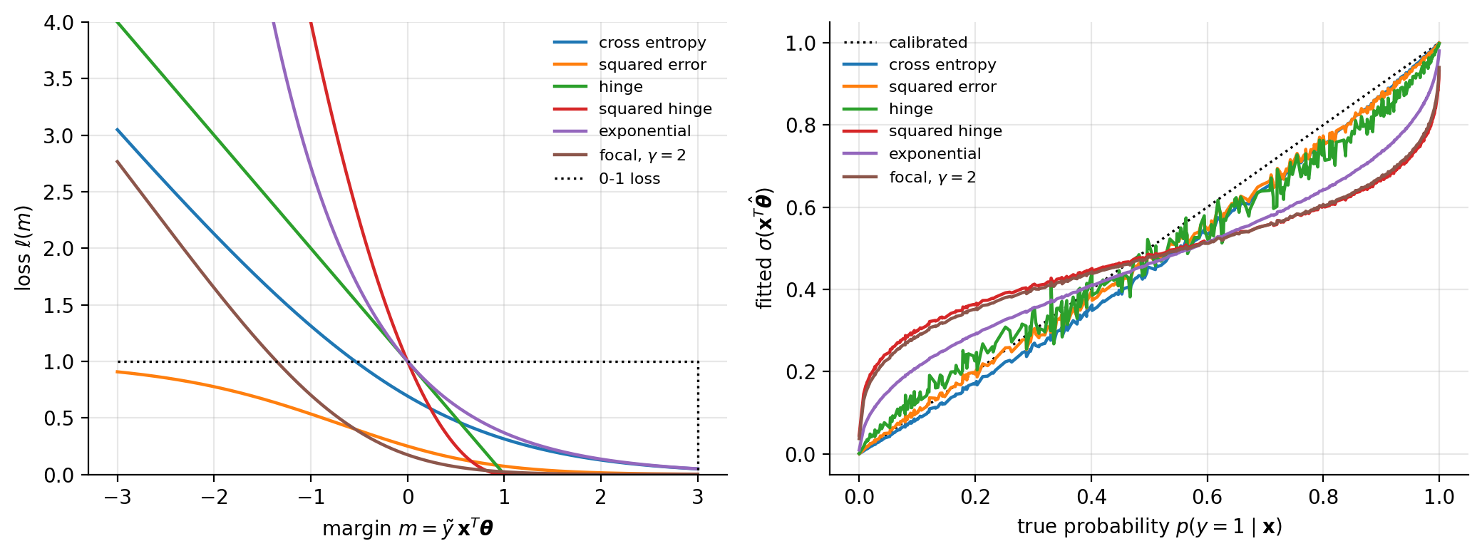
Figure 5.9: Left: the loss functions of Table 5.2 against the margin, for a point of class \(\tilde y=+1\); the 0–1 loss is dotted. Right: the probability \(\sigma(\bm{x}^{T}\hat{\bm{\theta}})\) obtained by minimising each loss with a linear model on \(400\) points drawn from a true logistic model, plotted against the true probability. The cross entropy and the squared error follow the diagonal; the exponential loss recovers half the log-odds, so its curve is the diagonal compressed towards \(\tfrac12\); the squared hinge and the focal loss are compressed further; the hinge loss does not estimate a probability at all.
A few features of the picture are worth pointing out before the algebra. All the surrogates agree on the sign of what they want – push the margin positive – and differ in how hard they push and where they stop. The hinge loss is exactly zero once \(m\ge1\), so points comfortably on the right side exert no force whatever; that is what will make support vectors in Chapter 6. The logistic and exponential losses never reach zero and keep rewarding larger margins, exponentially weakly in the first case and linearly in the second; the exponential loss also punishes a large negative margin exponentially hard, which is the origin of AdaBoost’s known sensitivity to mislabelled points. The squared error and the focal loss flatten out for large negative margins, which is the vanishing-gradient problem of the notebox in Section Maximum likelihood and the cross-entropy seen again: a confidently wrong point produces almost no gradient.
5.10.2. What each loss estimates#
A loss function does two jobs. It has to be minimised, which is a matter of convexity and smoothness, and its minimiser has to mean something. The second question has a clean answer, because in the limit of infinite data the fit at each \(\bm{x}\) minimises the expected loss there. Fix a point with true class probability \(\eta=p(y=1\mid\bm{x})\) and ask which value of the linear predictor \(t\) minimises
For a margin loss \(\ell(t,1)=\ell(t)\) and \(\ell(t,0)=\ell(-t)\). If the minimiser \(t^{*}\) has the sign of \(2\eta-1\), the surrogate is classification-calibrated [bartlett2006]: minimising it recovers the Bayes decision rule of the 0–1 loss. If, further, \(\sigma(t^{*})=\eta\) – or some fixed, invertible function of \(t^{*}\) equals \(\eta\) – the surrogate is a proper scoring rule [brier1950,gneiting2007] and the model’s output can be read as a probability.
Proposition 5.1 (Pointwise minimisers of the classification losses)
For \(0<\eta<1\) the minimiser of Eq. (5.50) is
All five are classification-calibrated. The logistic and squared-error losses are proper; the exponential and squared-hinge losses determine \(\eta\) through \(\sigma(2t^{*})\) and \((t^{*}+1)/2\) respectively; the hinge loss carries no information about \(\eta\) beyond its sign.
Proof
Each is a one-variable minimisation. For the logistic loss, \(L(t)=\eta\log(1+e^{-t})+(1-\eta)\log(1+e^{t})\) and \(L'(t)=-\eta(1-\sigma(t))+(1-\eta)\sigma(t)=\sigma(t)-\eta\), which vanishes exactly at \(\sigma(t^{*})=\eta\); \(L''=\sigma(1-\sigma)>0\), so it is the minimum. For the squared error, \(L(t)=\eta(1-\sigma)^{2}+(1-\eta)\sigma^{2}\) with \(\sigma=\sigma(t)\), and \(L'(t)=2(\sigma-\eta)\,\sigma'(t)\); since \(\sigma'>0\) the only stationary point is again \(\sigma(t^{*})=\eta\), and \(L\to\eta\) or \(1-\eta\) at \(t\to\mp\infty\), both larger than the value \(\eta(1-\eta)\) at the stationary point, so it is the global minimum although \(L\) is not convex. For the exponential loss \(L(t)=\eta e^{-t}+(1-\eta)e^{t}\), \(L'(t)=-\eta e^{-t} +(1-\eta)e^{t}=0\) gives \(e^{2t^{*}}=\eta/(1-\eta)\), and \(\sigma(2t^{*})=e^{2t^{*}}/(1+e^{2t^{*}})=\eta\). For the squared hinge the minimiser lies in \([-1,1]\), where both hinges are active, \(L(t)=\eta(1-t)^{2}+(1-\eta)(1+t)^{2}\) and \(L'(t)=-2\eta(1-t)+2(1-\eta)(1+t) =2(t-(2\eta-1))\). For the hinge, \(L(t)=\eta\max(0,1-t)+(1-\eta)\max(0,1+t)\) is piecewise linear with slope \(-\eta+(1-\eta)=1-2\eta\) on \([-1,1]\), slope \(1-\eta>0\) for \(t>1\) and slope \(-\eta<0\) for \(t<-1\); it is therefore minimised at \(t=1\) if \(\eta>\tfrac12\) and at \(t=-1\) if \(\eta<\tfrac12\), and the value at the minimum, \(2\min(\eta,1-\eta)\), depends on \(\eta\) but its location does not. In every case \(\mathrm{sign}(t^{*})=\mathrm{sign}(2\eta-1)\). \qed
The proposition is what the right panel of Fig. 5.9
shows empirically, and it explains a common misuse. A support vector machine
does not produce probabilities, and passing its decision function through a
sigmoid produces numbers that are systematically too close to \(\tfrac12\) –
which is why scikit-learn fits a separate logistic regression on top
of the SVM output when probabilities are requested (Platt scaling). A model
trained with the exponential loss must be read through \(\sigma(2t)\), not
\(\sigma(t)\); that is why the AdaBoost of Chapter 7 outputs
half the log-odds. And the focal loss [lin2017],
which multiplies each cross-entropy term by a factor that vanishes for well-classified points and thereby concentrates the gradient on the hard and the rare ones, is deliberately not proper: its minimiser is pushed towards \(\tfrac12\) (Exercise at the end of the chapter), so a detector trained with it must be recalibrated before its scores are read as probabilities. The cross entropy is the only member of the family that is convex, proper, and free of the vanishing-gradient defect, and that is the whole case for it; but each of the others buys something in exchange, and the following code makes it possible to see what without deriving a single derivative.
5.10.3. One program for every loss#
The class of Section An implementation hard-wired the cross-entropy gradient (5.17). With automatic differentiation the loss becomes a plain Python function of the linear predictor and the label, the cost is its mean over the data plus the penalty of Eq. (5.23), and JAX supplies the gradient – and, if wanted, the Hessian – of whatever we wrote. Trying a new loss means writing one line.
import jax
jax.config.update("jax_enable_x64", True)
import jax.numpy as jnp
import numpy as np
from jax import grad, jit, hessian
from jax.nn import sigmoid, softplus, log_sigmoid

# Every loss is a function of the linear predictor t = x^T theta and the label
# y in {0, 1}, evaluated pointwise; softplus(t) = log(1 + e^t) is the stable
# form of Eq. (5.crossentropycompact), log_sigmoid(t) = log sigma(t).
def cross_entropy(t, y):
    return softplus(t) - y * t                          # Eq. (5.logisticloss)

def squared_error(t, y):
    return (y - sigmoid(t))**2                          # the Brier score

def hinge(t, y):
    return jnp.maximum(0.0, 1.0 - (2*y - 1) * t)        # margin m = (2y-1) t

def squared_hinge(t, y):
    return jnp.maximum(0.0, 1.0 - (2*y - 1) * t)**2

def exponential(t, y):
    return jnp.exp(-(2*y - 1) * t)

def focal(t, y, gamma=2.0):                             # Eq. (5.focal)
    p = sigmoid(t)
    return -(y * (1 - p)**gamma * log_sigmoid(t)
             + (1 - y) * p**gamma * log_sigmoid(-t))

LOSSES = {"cross entropy": cross_entropy, "squared error": squared_error,
          "hinge": hinge, "squared hinge": squared_hinge,
          "exponential": exponential, "focal (gamma=2)": focal}

def cost(theta, X, y, loss, lmbda=0.0):
    """Mean loss over the data plus an l2 penalty that spares the intercept."""
    return jnp.mean(loss(X @ theta, y)) + lmbda * jnp.sum(theta[1:]**2)

def fit(loss, X, y, gamma=0.5, epochs=3000, lmbda=0.0):
    """Gradient descent, Eq. (5.gd), with the gradient supplied by JAX."""
    c = lambda th: cost(th, X, y, loss, lmbda)
    step = jit(lambda th: th - gamma * grad(c)(th))
    theta = jnp.zeros(X.shape[1])
    for _ in range(epochs):
        theta = step(theta)
    return theta

def newton(loss, X, y, iters=10, lmbda=1e-8):
    """Newton-Raphson, Eq. (5.newtonabstract), with the Hessian from JAX."""
    c = lambda th: cost(th, X, y, loss, lmbda)
    g, H = jit(grad(c)), jit(hessian(c))
    theta = jnp.zeros(X.shape[1])
    for _ in range(iters):
        theta = theta - jnp.linalg.solve(H(theta), g(theta))
    return theta
Before using it on anything, we check the machinery against the hand-derived results of Section Gradients, the Hessian and convexity: the automatic gradient of the cross entropy must be \(-\bm{X}^{T}(\bm{y}-\bm{p})/n\) and its automatic Hessian must be \(\bm{X}^{T}\bm{W}\bm{X}/n\). The data are drawn from a true logistic model, so that we can afterwards ask not only whether each loss classifies well but whether it estimates the right probabilities.
rng = np.random.default_rng(2024)
n = 400
X = jnp.asarray(np.c_[np.ones(n), rng.normal(size=(n, 2))])
theta_true = jnp.array([0.5, 2.0, -1.0])
p_true = sigmoid(X @ theta_true)                       # the truth we try to recover
y = jnp.asarray((rng.random(n) < np.asarray(p_true)).astype(float))

theta0 = jnp.array([0.1, -0.3, 0.2])
g_ad = grad(cost)(theta0, X, y, cross_entropy)
g_hand = -X.T @ (y - sigmoid(X @ theta0)) / n                 # Eq. (5.gradient)
print("gradient: max |AD - hand| =", float(jnp.max(jnp.abs(g_ad - g_hand))))

p0 = sigmoid(X @ theta0)
H_ad = hessian(cost)(theta0, X, y, cross_entropy)
H_hand = X.T @ ((p0 * (1 - p0))[:, None] * X) / n              # Eq. (5.hessian)
print("Hessian:  max |AD - hand| =", float(jnp.max(jnp.abs(H_ad - H_hand))))

print("Newton :", newton(cross_entropy, X, y))
print("GD     :", fit(cross_entropy, X, y))
gradient: max |AD - hand| = 2.220446049250313e-16
Hessian:  max |AD - hand| = 3.0531133177191805e-16
Newton : [ 0.26067864  1.93734364 -1.00125907]
GD     : [ 0.26067869  1.93734439 -1.00125944]
Both derivatives agree with Eqs. (5.17) and (5.19)
to rounding, and Newton’s method built from jax.hessian lands in ten
iterations where three thousand steps of gradient descent land, the two
differing in the seventh digit only through the tiny ridge term that keeps
the Hessian invertible. Now the loop that
motivated the section:
def evaluate(theta):
    p = sigmoid(X @ theta)
    accuracy = float(jnp.mean((p > 0.5) == (y > 0.5)))
    calibration = float(jnp.mean(jnp.abs(p - p_true)))    # mean |p_hat - p_true|
    return accuracy, calibration

print(f"{'loss':16s} {'theta':26s} accuracy   mean |p_hat - p_true|")
for name, loss in LOSSES.items():
    theta = fit(loss, X, y)
    acc, cal = evaluate(theta)
    print(f"{name:16s} {np.array2string(np.asarray(theta), precision=2):26s}"
          f" {acc:.3f}      {cal:.3f}")
print("true            ", np.asarray(theta_true))
loss             theta                      accuracy   mean |p_hat - p_true|
cross entropy    [ 0.26  1.94 -1.  ]        0.790      0.032
squared error    [ 0.32  1.82 -0.97]        0.790      0.024
hinge            [ 0.28  1.53 -0.89]        0.792      0.043
squared hinge    [ 0.1   0.69 -0.36]        0.795      0.156
exponential      [ 0.11  1.06 -0.53]        0.780      0.103
focal (gamma=2)  [ 0.09  0.74 -0.38]        0.782      0.149
true             [ 0.5  2.  -1. ]
The accuracies are all within a percent of one another, and of the Bayes rate of \(0.79\) for this problem: every loss in the table is classification-calibrated, as Proposition 5.1 says, and all of them find essentially the same decision boundary. The probabilities are another matter, and the last column is Proposition 5.1 in numbers. The two proper losses recover the true parameters up to sampling error. The exponential loss returns \((0.11,1.06,-0.53)\), which is the true vector halved – Eq. (5.53), \(t^{*}=\tfrac12\log[\eta/(1-\eta)]\) – and its probabilities are correct once read through \(\sigma(2t)\). The squared hinge and the focal loss compress the parameters by a factor of about three and their \(\sigma(t)\) is badly miscalibrated, while their accuracy is unharmed. Nothing about these conclusions required a derivative, and the reader can now add a loss to the dictionary – an asymmetric one that penalises false negatives more than false positives, a class-weighted cross entropy, a Huberised hinge – and have the answer in seconds.
Machine learning connection
The pattern of this section is how
loss functions are actually developed. A practitioner writes the loss as a
few lines of framework code, lets the framework differentiate it, and judges
the result empirically; the theoretical questions – is it convex, is it
proper, is it classification-calibrated – are asked afterwards, and often
answered by exactly the pointwise argument of
Proposition 5.1. Every framework in the later chapters
(PyTorch, TensorFlow, JAX) offers the losses of
Table 5.2 as library functions, but nothing in them is
special: torch.nn.BCEWithLogitsLoss is softplus(t) - y*t,
and a loss the library does not offer is one line away. The one practical
rule is the one used above: write losses in terms of the logit \(t\) and the
stable primitives softplus and log_sigmoid, never in terms
of \(\log\sigma(t)\) computed literally, for the reasons of
Section Optimising the cross entropy.
5.11. Kernel logistic regression#
Logistic regression produces a linear decision boundary, and Section Kernel methods: regression without coordinates showed how to remove that restriction from Ridge regression without ever constructing the enlarged feature space. The same construction applies here, and it applies for the same reason: by Theorem 3.12 the reason had nothing to do with the squared error.
5.11.1. The problem, and what the representer theorem gives#
Replace the linear predictor \(\bm{x}^{T}\bm{\theta}\) by a function \(f\in\mathcal{H}\), the reproducing kernel Hilbert space of a kernel \(k\), and penalise its norm:
with \(\sigma\) the logistic function (5.3) and \(y_i\in\{0,1\}\). The data-fitting term is the cross entropy (5.13) with \(\bm{x}_i^{T}\bm{\theta}\) replaced by \(f(\bm{x}_i)\), and the penalty is the \(\ell_2\) penalty of Section More predictors, and regularisation measured in \(\mathcal{H}\) rather than in \(\mathbb{R}^{p}\).
Theorem 3.12 applies immediately: the loss depends on \(f\) only through its values at the training points, and \(\Omega(t)=\tfrac{\lambda}{2}t^{2}\) is strictly increasing. The minimiser is therefore
the second identity because \(\|f\|^{2}=\sum_{ij}\alpha_i\alpha_j\langle k(\bm{x}_i,\cdot), k(\bm{x}_j,\cdot)\rangle\), which is \(\sum_{ij}\alpha_i\alpha_jK_{ij}\). The infinite-dimensional problem has become the \(n\)-dimensional one
5.11.2. Gradient, Hessian and kernel IRLS#
The derivatives are obtained from Section Gradients, the Hessian and convexity by the substitution \(\bm{X}\rightarrow\bm{K}\), which is the whole of the work: the chain rule sees \(\bm{K}\bm{\alpha}\) exactly as it saw \(\bm{X}\bm{\theta}\). Differentiating Eq. (5.59) and using Eq. (1.28) for the penalty,
to be compared with Eq. (5.17), and
with \(\bm{W}\) the same diagonal matrix (5.18) of weights \(p_i(1-p_i)\). Since \(\bm{K}\) is positive semi-definite, so is Eq. (5.61) by the argument of Eq. (5.20), and the problem is convex; for \(\lambda>0\) and \(\bm{K}\) positive definite it is strictly convex, so the minimiser is unique.
Newton’s method now takes a form worth deriving, because it turns out to be the exact analogue of the iteratively reweighted least squares of Eq. (5.34). Assume \(\bm{K}\) invertible and factor it out of Eq. (5.61) on the left, \(\bm{K}\bm{W}\bm{K}+\lambda\bm{K}=\bm{K}(\bm{W}\bm{K}+\lambda\bm{I})\). The Newton step \(\bm{\Delta}=-\bm{H}^{-1}\bm{g}\) is then
the inverse Gram matrices cancelling. Adding \(\bm{\alpha}\) and collecting,
where the working response
is the adjusted response defined just above Eq. (5.34), with \(\bm{X}\bm{\theta}\) replaced by \(\bm{K}\bm{\alpha}\). Multiplying Eq. (5.63) through by \(\bm{W}^{-1}\) inside the inverse gives the form to remember,
Compare Eq. (5.65) with the kernel ridge regression (3.84), \(\bm{\alpha}=(\bm{K}+\lambda\bm{I})^{-1}\bm{y}\). They differ in two places only: the targets \(\bm{y}\) have become the working response \(\bm{z}\), and the uniform penalty \(\lambda\bm{I}\) has become the per-observation penalty \(\lambda\bm{W}^{-1}\), which is small where the model is uncertain and large where it is confident. Kernel logistic regression is iteratively reweighted kernel ridge regression, exactly as ordinary logistic regression is iteratively reweighted least squares. The parallel of Section Optimising the cross entropy is complete, and it is not a coincidence but a consequence of Theorem 3.12: the same substitution that turned least squares into kernel ridge regression turns each reweighted step into a reweighted kernel step.
import numpy as np

def kernel_irls(K, y, lmbda, n_iter=100, tol=1e-13, jitter=1e-12):
    """Kernel logistic regression by Newton's method, Eq. (5.kirls).

    Each iteration is a kernel ridge regression, Eq. (3.krr), on the working
    response z with the per-observation penalty lambda / W_ii.
    """
    n = len(y)
    alpha = np.zeros(n)
    for _ in range(n_iter):
        f = K @ alpha
        p = sigmoid(f)
        w = np.maximum(p * (1.0 - p), 1e-10)          # W_ii, Eq. (5.Wmatrix)
        z = f + (y - p) / w                           # Eq. (5.kworking)
        new = np.linalg.solve(K + lmbda * np.diag(1.0 / w)
                              + jitter * np.eye(n), z)
        if np.linalg.norm(new - alpha) < tol:
            return new
        alpha = new
    return alpha


def kernel_logistic_predict(alpha, Xtrain, Xnew, gamma):
    """p(y=1|x) = sigma(sum_j alpha_j k(x_j, x))."""
    return sigmoid(gaussian_kernel(Xnew, Xtrain, gamma) @ alpha)
The \verb!jitter! is there because \(\bm{K}\) for a Gaussian kernel is positive definite in exact arithmetic and can be numerically singular when two training points nearly coincide; adding \(10^{-12}\) to the diagonal is the standard remedy and changes nothing that matters.
5.11.3. The method, verified#
The test problem is one that no linear boundary can solve at all: \(120\) points in the plane, labelled by whether they fall inside a disc, with five per cent of the labels flipped. Newton’s method on Eq. (5.65) with a Gaussian kernel converges in six iterations, and the step lengths show the quadratic rate of Section Optimising the cross entropy unmistakably:
    iteration        cost          ||delta alpha||
            1    56.8201866189          3.602e+00
            2    56.4403059843          2.888e-01
            3    56.4394190411          1.438e-02
            4    56.4394190342          3.825e-05
            5    56.4394190342          3.059e-10
            6    56.4394190342          2.018e-15
Each step length is roughly the square of the one before once the iterate is close, which is what distinguishes Newton’s method from the linearly convergent gradient descent of Chapter 4. Plain gradient descent on the same objective reaches the same minimum, more slowly: it agrees with the Newton solution to \(9.1\times10^{-5}\) in the fitted function, which is its own convergence tolerance and not a disagreement about the answer.
The more searching test is against the primal problem. With the quadratic kernel \((\bm{x}^{T}\bm{x}'+1)^{2}\) the feature map is only six-dimensional, so the same fit can be obtained by ordinary penalised logistic regression in that map and the two compared:
  max |k(x,x') - phi(x).phi(x')|: 4.263e-14
  max |f_kernel(x) - f_primal(x)| on 400 test points: 6.004e-13
  ||theta_primal||^2 = 13.2542532295,   alpha^T K alpha = 13.2542532295

  scikit-learn in the same map, C = 1/lambda:
    max |theta_ours - theta_sklearn| : 9.498e-09
    max |f_ours - f_sklearn| on test : 7.232e-08
The third line is the one to notice. The primal penalty
\(\|\bm{\theta}\|_2^{2}\) and the dual penalty
\(\bm{\alpha}^{T}\bm{K}\bm{\alpha}\) agree to ten digits because they are the
same number written twice: both are \(\|f\|_{\mathcal{H}}^{2}\), the squared norm
of one function in one space. Note also the conversion to
scikit-learn’s convention, \(C=1/\lambda\), warned about in
Section More predictors, and regularisation; with it, three independent implementations
agree to the tolerance of the least accurate.
5.11.4. What the coefficients are#
Setting Eq. (5.60) to zero gives a fact about kernel logistic regression that is easy to miss and explains a good deal.
Proposition 5.2 (The coefficients are the residuals)
If \(\bm{K}\) is invertible, the minimiser of Eq. (5.59) satisfies
Proof
Stationarity is \(\bm{K}[(\bm{p}-\bm{y})+\lambda\bm{\alpha}]=\bm{0}\) by Eq. (5.60). Multiplying by \(\bm{K}^{-1}\) gives \(\lambda\bm{\alpha}=\bm{y}-\bm{p}\). \qed
The weight a training point carries in the fitted function (5.58) is its own residual divided by the penalty. Points the model already predicts correctly and confidently have small residuals and contribute little; points it gets wrong contribute much. But \(p_i\) is a logistic probability and lies strictly between zero and one, so the residual \(y_i-p_i\) is never exactly zero: every training point contributes something, and \(\bm{\alpha}\) is dense.
   lambda   max |alpha - (y-p)/lambda|   non-zero alpha of 120   |alpha|_min
     0.10                   1.471e-11                 120   2.065e-02
     1.00                   1.477e-13                 120   6.360e-02
    10.00                   1.422e-15                 120   3.472e-02
This is the practical drawback of the method and the reason it is less used than its two neighbours. Prediction costs \(n\) kernel evaluations no matter how easy the problem is, where a support vector machine on the same data would retain a fraction of the points. Section One penalty, three losses shows that this contrast is not an accident of the two algorithms but a theorem about their losses, and that Eq. (5.66) is one instance of a formula covering all three of the kernel methods in this book.
Machine learning connection
What kernel logistic regression buys over a support vector machine is a calibrated probability. The output of Eq. (5.58) passed through the sigmoid is an estimate of \(p(y=1\mid\bm{x})\) obtained by maximising a likelihood, so it can be thresholded at a cost-sensitive value, combined with other probabilities, or fed to a decision rule – all of which the signed distance produced by Eq. (6.33) cannot support without an extra calibration step fitted on held-out data. Against that stands the dense \(\bm{\alpha}\) of Proposition 5.2 and the \(\bigO(n^{3})\) cost of each Newton step. The choice between them is the usual one in this book: a probability, or a sparse representation, but not both from the same fit.
5.11.5. The penalty, measured#
Everything Section More predictors, and regularisation said about the penalty holds here, with one addition: the kernel supplies enough flexibility to interpolate the training data exactly, so the penalty is no longer optional. Running the same fit across six decades:
   lambda    train accuracy   test accuracy   alpha^T K alpha
     0.001           0.9500          0.9300         5027.0188
     0.010           0.9417          0.9275          696.1591
     0.100           0.9500          0.9375          144.9844
     1.000           0.9333          0.9400           22.4656
    10.000           0.8750          0.9150            1.0326
   100.000           0.8667          0.8700            0.0146
The best test accuracy is at \(\lambda=1\), in the interior, with the norm of the fitted function falling by five orders of magnitude across the range. At \(\lambda=10^{-3}\) the model is reproducing the five per cent of deliberately flipped labels and pays for it on the test set; at \(\lambda=100\) it has been flattened towards a constant. This is Eq. (2.52) once more, and it is why the kernel and the penalty must be chosen together by the cross-validation of Section Cross-validation and never by the training error.
5.12. Measuring the quality of a classifier#
The mean squared error and \(R^{2}\) of Section Measures of quality are meaningless for a classifier. We need measures appropriate to discrete outcomes, and it turns out that no single number will do.
The confusion matrix. Everything starts here. For two classes, cross-tabulating the true label against the predicted one gives four counts:
the true positives, false negatives, false positives and true negatives. Every scalar measure below is a function of these four numbers, and reporting the matrix itself is almost always more informative than reporting any of them.
Accuracy, and why it misleads. The obvious measure is the fraction correctly classified,
with \(I\) the indicator function. Accuracy is the right measure when the classes are balanced and the two kinds of error are equally costly. It is badly misleading otherwise. If one in a thousand transactions is fraudulent, the classifier that declares everything legitimate achieves \(99.9\%\) accuracy while being entirely useless. Always compare an accuracy against the proportion of the majority class, which is the score obtained for free.
Precision and recall. Separating the two kinds of error gives
Precision asks: of the samples flagged positive, what fraction really were? Recall asks: of the samples that really were positive, what fraction did we find? The two trade off against each other through the decision threshold. Lowering the threshold flags more samples, catching more of the true positives – recall rises – at the cost of more false alarms – precision falls. Which matters more is a question about the application and not about the model: in screening for a serious disease a false negative is far worse than a false positive, so recall dominates; in flagging emails as spam the reverse holds. The harmonic mean of the two,
is the usual compromise; the harmonic mean rather than the arithmetic one because it is small unless both are large.
ROC and AUC. Because logistic regression outputs a probability rather than a decision, the threshold is ours to choose, and a fair assessment should not depend on one arbitrary choice. The receiver operating characteristic curve plots the true positive rate \(\mathrm{TP}/(\mathrm{TP}+\mathrm{FN})\), which is the recall, against the false positive rate \(\mathrm{FP}/(\mathrm{FP}+\mathrm{TN})\), as the threshold sweeps from one to zero. A perfect classifier passes through the top-left corner; a classifier that ranks at random gives the diagonal. The area under the curve, the AUC, summarises the whole sweep in a single number, and it has a clean interpretation: it is the probability that a randomly chosen positive sample receives a higher score than a randomly chosen negative one. An AUC of \(0.5\) is chance and \(1.0\) is perfect. Since AUC depends only on the ranking, it is insensitive to class imbalance in a way accuracy is not.
import numpy as np

def confusion_matrix(y_true, y_pred):
    """Return TP, FN, FP, TN for binary labels in {0, 1}."""
    tp = int(np.sum((y_true == 1) & (y_pred == 1)))
    fn = int(np.sum((y_true == 1) & (y_pred == 0)))
    fp = int(np.sum((y_true == 0) & (y_pred == 1)))
    tn = int(np.sum((y_true == 0) & (y_pred == 0)))
    return tp, fn, fp, tn


def classification_report(y_true, y_pred):
    tp, fn, fp, tn = confusion_matrix(y_true, y_pred)
    accuracy = (tp + tn) / (tp + tn + fp + fn)
    precision = tp / (tp + fp) if tp + fp else 0.0
    recall = tp / (tp + fn) if tp + fn else 0.0
    f1 = (2 * precision * recall / (precision + recall)
          if precision + recall else 0.0)
    return dict(accuracy=accuracy, precision=precision, recall=recall, f1=f1)


def roc_auc(y_true, scores):
    """AUC as the probability that a positive outranks a negative."""
    order = np.argsort(scores)
    ranks = np.empty(len(scores), dtype=float)
    ranks[order] = np.arange(1, len(scores) + 1)
    n_pos = int(np.sum(y_true == 1))
    n_neg = len(y_true) - n_pos
    return (np.sum(ranks[y_true == 1]) - n_pos * (n_pos + 1) / 2) / (n_pos * n_neg)
Machine learning connection
The cross entropy is the loss we optimise; accuracy, \(F_1\) and AUC are what we report. They are not the same and cannot be, because accuracy is a step function of the parameters – flat almost everywhere, with jumps where a prediction crosses the threshold – so its gradient is zero wherever it is defined and no method of Chapter 4 could minimise it. The cross entropy is a smooth surrogate that is minimised in roughly the same place. This split between a differentiable training objective and a non-differentiable evaluation metric runs through all of machine learning, and it is worth being explicit that a model with the lower cross entropy does not automatically have the higher accuracy. It also explains why, when the classes are severely imbalanced, one often weights the cross entropy by class frequency: to move the minimum of the surrogate closer to the optimum of the metric one actually cares about.
5.13. The Wisconsin breast cancer data#
We close with a real data set. The Wisconsin breast cancer data contain \(569\)
samples, each described by \(30\) features computed from a digitised image of a
fine-needle aspirate of a breast mass – radius, texture, perimeter, area,
smoothness and so on, each in three variants – and each labelled malignant or
benign. It is a natural test for a binary classifier and is included with
scikit-learn.
import numpy as np
from sklearn.datasets import load_breast_cancer
from sklearn.model_selection import train_test_split, cross_validate
from sklearn.preprocessing import StandardScaler
from sklearn.pipeline import make_pipeline
from sklearn.linear_model import LogisticRegression

cancer = load_breast_cancer()
X_train, X_test, y_train, y_test = train_test_split(
    cancer.data, cancer.target, random_state=0)
print(X_train.shape, X_test.shape)

# Scaling inside the pipeline, so it is refitted on each training fold
logreg = make_pipeline(StandardScaler(), LogisticRegression(max_iter=5000))
logreg.fit(X_train, y_train)

print(f"test accuracy: {logreg.score(X_test, y_test):.3f}")
scores = cross_validate(logreg, X_train, y_train, cv=10)["test_score"]
print(f"cross-validated accuracy: {scores.mean():.3f} +/- {scores.std():.3f}")
The scaler is not decoration. The thirty features differ enormously in
scale – the mean area is around \(655\) while the mean smoothness is around
\(0.096\), a ratio of some four orders of magnitude, and the ratio of the
largest to the smallest standard deviation across the thirty columns exceeds
\(10^{5}\) – so by Section More predictors, and regularisation the default \(\ell_2\)
penalty would fall almost entirely on the small-scale features, and by
Section The learning rate and the condition number the optimisation would be badly conditioned.
Placing the scaler inside a Pipeline ensures it is refitted on each
training fold, honouring the discipline of
Section Cross-validation.
Inspecting the features. Before fitting anything it is worth looking at the data. Plotting, for each feature, the histograms of the two classes superimposed shows immediately which features separate them.
import matplotlib.pyplot as plt
import pandas as pd

cancerpd = pd.DataFrame(cancer.data, columns=cancer.feature_names)
malignant = cancer.data[cancer.target == 0]
benign = cancer.data[cancer.target == 1]

fig, axes = plt.subplots(15, 2, figsize=(10, 20))
ax = axes.ravel()
for i in range(30):
    _, bins = np.histogram(cancer.data[:, i], bins=50)
    ax[i].hist(malignant[:, i], bins=bins, alpha=0.5)
    ax[i].hist(benign[:, i], bins=bins, alpha=0.5)
    ax[i].set_title(cancer.feature_names[i])
    ax[i].set_yticks(())
ax[0].set_xlabel("Feature magnitude")
ax[0].set_ylabel("Frequency")
ax[0].legend(["Malignant", "Benign"], loc="best")
fig.tight_layout()
plt.show()

# The correlation matrix of Section 1.covariance, computed with pandas
correlations = cancerpd.corr()
plt.figure(figsize=(10, 9))
plt.imshow(correlations, vmin=-1, vmax=1, cmap="RdBu_r")
plt.colorbar(); plt.title("Correlation matrix of the features")
plt.show()
The correlation matrix repays study, and it connects directly to Chapter 1. Several groups of features are almost perfectly correlated – radius, perimeter and area are essentially the same measurement three times over, since a roughly circular region has perimeter and area determined by its radius. By Section Rank, the pseudoinverse and ill-conditioned design matrices this makes the design matrix nearly rank deficient, so the individual coefficients are poorly determined even though the predictions are not. Three remedies are available and all appear in this book: penalise with \(\ell_2\), as the default settings do; select with \(\ell_1\), which will keep one member of each correlated group; or reduce the dimension first with the principal component analysis of Section Principal component analysis. The point to carry away is that a high accuracy on this data set does not license a statement about which feature matters, because the data cannot distinguish the members of a correlated group.
from sklearn.metrics import (confusion_matrix, classification_report,
                             roc_auc_score, RocCurveDisplay)

y_pred = logreg.predict(X_test)
y_proba = logreg.predict_proba(X_test)[:, 1]

print(confusion_matrix(y_test, y_pred))
print(classification_report(y_test, y_pred,
                            target_names=cancer.target_names))
print(f"AUC: {roc_auc_score(y_test, y_proba):.4f}")

RocCurveDisplay.from_predictions(y_test, y_proba)
plt.show()
The run above gives a test accuracy of \(0.958\), a cross-validated accuracy on the training set of \(0.981\pm0.025\), and an AUC of \(0.9914\). The confusion matrix on the \(143\) test samples is
with rows the true class (malignant, benign) and columns the predicted one.
These numbers should be read with the cautions of Section Measuring the quality of a classifier in mind. An accuracy of \(0.958\) sounds impressive until one notices that \(62.7\%\) of the samples are benign, so the classifier that predicts “benign” unconditionally already scores \(0.629\); the model has removed about nine tenths of the remaining error, which is the honest way to state the achievement. The AUC of \(0.9914\) is the more informative summary, being independent of both the threshold and the class balance.
The confusion matrix is more informative still, because it separates the two kinds of error: three malignant cases were predicted benign and three benign cases malignant. In a screening context those are not equivalent, and one would deliberately move the threshold below \(0.5\) to reduce the first at the cost of increasing the second – trading precision for recall, exactly as discussed in Section Measuring the quality of a classifier. Note finally that the cross-validated accuracy (\(0.981\)) exceeds the test accuracy (\(0.958\)); with \(143\) test samples the standard error of the latter is about \(0.017\) by Eq. (2.24), so the difference is within about one and a half standard errors and should not be over-interpreted.
Figure 5.10 shows the two summaries that matter. The ROC curve hugs the top-left corner, giving an AUC of \(0.9914\); because the AUC depends only on the ranking of the predicted probabilities, it is unaffected by the class imbalance that makes the raw accuracy flattering. The confusion matrix is the more actionable object: it separates the three malignant cases predicted benign from the three benign cases predicted malignant, and in a screening context those two numbers carry very different costs.
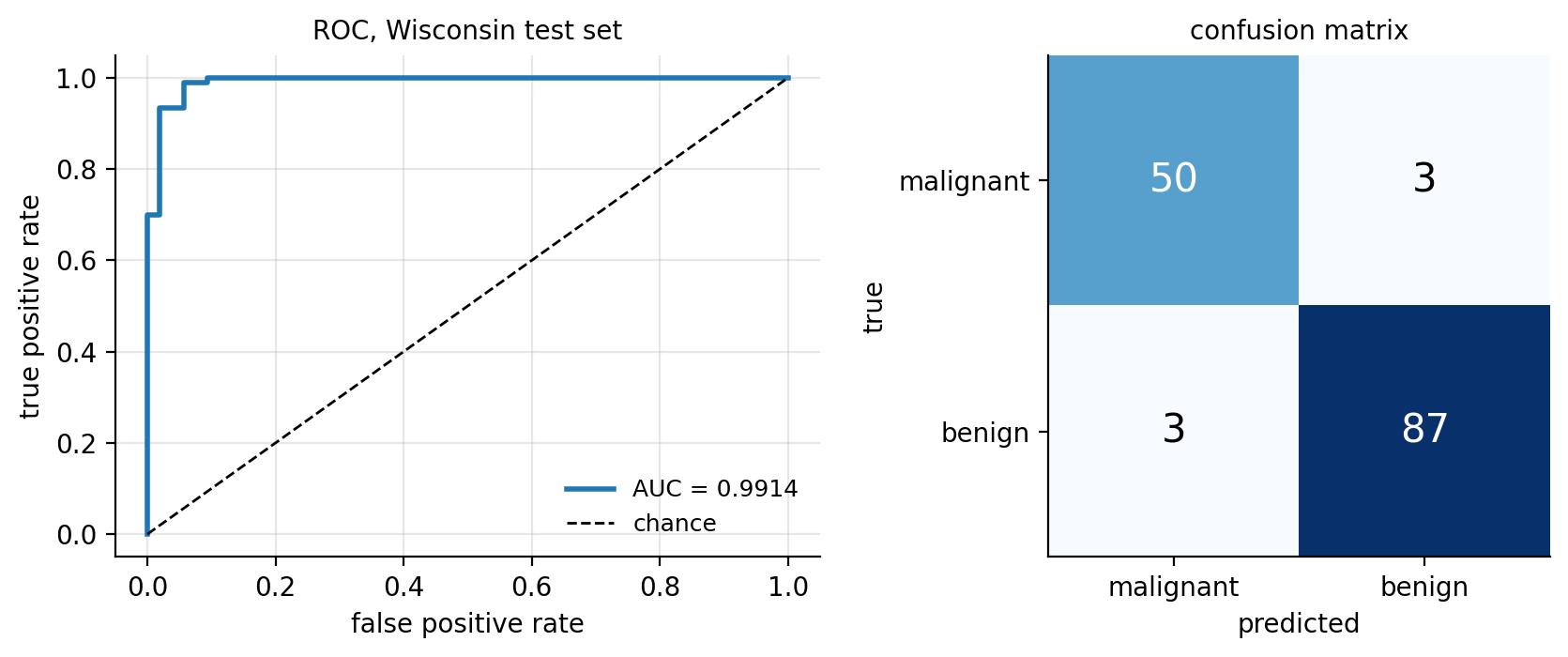
Figure 5.10: Logistic regression on the Wisconsin test set. Left: the ROC curve, with AUC \(=0.9914\). Right: the confusion matrix, whose off-diagonal entries are the two kinds of error and are not equally costly.
5.14. Summary and the programs#
Logistic regression is the bridge between the linear models of Chapter 3 and the neural networks of the next chapter, and it is worth setting out how little had to change and how much followed.
The model changed by one function. We kept the linear predictor \(\bm{x}^{T}\bm{\theta}\) and passed it through the sigmoid (5.3), which confines the output to \((0,1)\) so that it can be read as a probability. Equivalently, by Eq. (5.10), we modelled the log-odds as linear while the probability itself is not.
The loss followed from the model rather than being chosen. Repeating the maximum-likelihood argument of Section Deriving least squares from a probability distribution with Bernoulli rather than Gaussian observations produced the cross entropy (5.13), just as the notebox there predicted. This is worth remembering as a general principle: specify the distribution of the target and the loss function is determined. It is not, however, the only usable loss: Section Other loss functions, and automatic differentiation placed it in the family of margin-based surrogates for the 0–1 loss, alongside the hinge loss of the coming support vector machine and the exponential loss of boosting, and Proposition 5.1 showed that all of them find the same decision boundary while only the proper ones – cross entropy and squared error – estimate the class probability itself. With automatic differentiation, switching between them cost one line of code.
The mathematics then ran parallel to Chapter 3 throughout. The gradient is \(-\bm{X}^{T}(\bm{y}-\bm{p})\), design matrix against residual, exactly as in least squares with the linear prediction replaced by the probability. The Hessian is \(\bm{X}^{T}\bm{W}\bm{X}\) rather than \(\bm{X}^{T}\bm{X}\), with weights \(p_i(1-p_i)\) that vanish for confidently classified points – so the fit is controlled by the points near the decision boundary. Positivity of those weights proves convexity, so Chapter 4 applies with its guarantees intact. What was lost is the closed form: the parameter appears inside a non-linear function and cannot be extracted, so we optimise numerically, by gradient descent for large problems and by Newton-Raphson – which is iteratively reweighted least squares, Eq. (5.34) – for small ones. For large problems, Section Stochastic gradient descent for logistic regression measured what Chapter 4 promised: on \(50\,000\) observations five epochs of minibatch SGD are worth a hundred of gradient descent, the adaptive methods add nothing on standardised features and an order of magnitude on unstandardised ones – they remove the column scales from the curvature but not from the distance each parameter has to travel, so that standardising still pays – and the accuracy saturates long before the cost.
Drawn as a diagram, Section Logistic regression as a single neuron, the model is a single artificial neuron – the perceptron with a sigmoid in place of the step – and the gradient is the delta rule (5.37), the residual times the input on each edge. The same diagram read backwards is the reverse sweep of automatic differentiation, Section The same algorithm by automatic differentiation, which produces \(\bm{X}^{T}(\bm{p}-\bm{y})\) in one pass at the cost of evaluating the cost itself; with more than one layer it is backpropagation.
A third extension removed the linearity altogether. By the representer theorem of Section Why the same trick works for any loss: the representer theorem the penalised problem in a reproducing kernel Hilbert space has a finite solution \(f=\sum_j\alpha_jk(\bm{x}_j,\cdot)\), and Newton’s method on it, Eq. (5.65), is iteratively reweighted kernel ridge regression – the same sentence as before with the design matrix replaced by the Gram matrix throughout. Proposition 5.2 then says that the coefficients are the residuals divided by the penalty, so they are never zero: kernel logistic regression buys a calibrated probability and pays for it with a predictor that involves every training point, which is the comparison Section One penalty, three losses completes.
Two extensions completed the picture. The softmax (5.27) generalises the sigmoid to \(K\) classes and preserves the gradient structure, and the penalties of Chapter 3 carry over unchanged, with the additional observation that some penalty is necessary when the classes are linearly separable. Finally, assessing a classifier needs a different vocabulary from assessing a regression: the confusion matrix and the measures built from it, with the standing warning that accuracy alone is uninformative when the classes are imbalanced.
The complete programs are collected in doc/BookML/BookPrograms:
kernel_logistic.py– kernel IRLS, Eq. (5.65), against gradient descent on the same objective, against the primal problem in an explicit feature map and againstscikit-learn; the residual identity of Proposition 5.2; and the penalty study of Section The penalty, measured.logistic_regression.py– the class of Section An implementation for the binary and multiclass cases, the synthetic data generators, and the numerically stable sigmoid and softmax of Eqs. (5.3) and (5.30), and the automatic-differentiation version of Section The same algorithm by automatic differentiation: the one-observation trace, the forward and reverse sweeps by hand and from JAX, and the forward-against- reverse timing.logistic_sgd.py– the listing of Section Stochastic gradient descent for logistic regression: the minibatch loop of Eq. (5.45) around the step function of Section Implementations, run as gradient descent, SGD with constant and decaying learning rates, AdaGrad, RMSProp and Adam on standardised and on raw features, reproducing Table 5.1; the figure scriptBookFigures/ch05_sgd_figures.pyadds the learning-rate grid behind Figures 5.6 and 5.7.logistic_losses_jax.py– the loss-agnostic trainer of Section One program for every loss: the six losses of Table 5.2 as one-line functions, gradient descent and Newton’s method with derivatives from JAX, the checks against Eqs. (5.17) and (5.19), and the accuracy-and-calibration comparison of Proposition 5.1.logreg_newton.py– Newton-Raphson and IRLS as in Eqs. (5.33) and (5.34), with a comparison of iteration counts against gradient descent and against the adaptive methods of Chapter 4.classification_metrics.py– the confusion matrix, accuracy, precision, recall, \(F_1\) and AUC of Section Measuring the quality of a classifier, checked againstscikit-learn.wisconsin.py– the complete analysis of Section The Wisconsin breast cancer data, including the feature histograms, the correlation matrix, the cross-validated accuracy and the ROC curve.
Each file runs as a script and reproduces the numbers quoted in this chapter. An executable version is available as a Jupyter notebook in the accompanying Jupyter-book.
Looking ahead. Logistic regression is a neural network with no hidden layer, Figure 5.4. Its linear predictor is a single artificial neuron, its sigmoid is that neuron’s activation function, its cross entropy is the loss used to train classification networks, and the minibatch loop of Section Stochastic gradient descent for logistic regression is the loop that will train them. The next chapter inserts layers between the input and the output, so that the features fed to the final sigmoid are themselves learned rather than given; the gradient of the last layer will be exactly Eq. (5.17), and backpropagation is the chain rule (1.51) carrying that gradient backwards through the preceding layers. Almost everything in this chapter will be reused.
5.15. Exercises#
5.15.1. Warm-up exercises#
Properties of the sigmoid. (a) Prove Eq. (5.4), \(1-\sigma(t)=\sigma(-t)\). (b) Prove Eq. (5.5), \(\sigma'=\sigma(1-\sigma)\), and show that the derivative attains its maximum value \(1/4\) at \(t=0\). (c) Verify Eq. (5.7), \(\tanh(t)=2\sigma(2t)-1\), and deduce the derivative of \(\tanh\) in terms of \(\tanh\) itself. (d) Show that the logit (5.6) is the inverse of the sigmoid.
The cross entropy from the likelihood. (a) Explain why the single expression \(p^{y_i}(1-p)^{1-y_i}\) correctly handles both \(y_i=0\) and \(y_i=1\). (b) Derive Eq. (5.13) from Eq. (5.11). (c) Derive the compact form (5.14) and explain why it is numerically preferable.
The gradient. (a) Derive Eqs. (5.15) and (5.16) by differentiating Eq. (5.14). (b) Assemble them into the matrix form (5.17). (c) Compare with the least-squares gradient (1.38) and state precisely what is the same and what differs.
Why not squared error (numerical). Consider one observation with \(y=1\) and a confidently wrong prediction, \(\sigma(t)=0.01\). (a) Compute the gradient with respect to \(t\) of the squared error \((y-\sigma(t))^{2}\) and of the cross entropy. (b) Repeat for \(\sigma(t)=0.5\) and \(\sigma(t)=0.99\). (c) Plot both gradients against \(t\) and explain, using the notebox of Section Maximum likelihood and the cross-entropy, why the cross entropy is preferred.
The Hessian and convexity. (a) Derive Eq. (5.19) from Eq. (5.17). (b) Prove positive semi-definiteness as in Eq. (5.20). (c) Show that adding an \(\ell_2\) penalty makes the Hessian positive definite, and explain why the problem is then strictly convex. (d) Show that \(W_{ii}\le 1/4\) and use this to justify the learning-rate bound quoted in Section Optimising the cross entropy.
Separability (numerical). Generate two classes that are perfectly separable in one dimension. (a) Fit an unpenalised logistic regression by gradient descent and plot \(\|\bm{\theta}\|\) against the iteration count. What happens? (b) Plot the cost against the iteration count. Does it converge? (c) Repeat with an \(\ell_2\) penalty and explain the difference.
Softmax. (a) Show that Eq. (5.27) reduces to Eqs. (5.8) and (5.9) when \(K=2\) and \(\bm{\theta}_0=\bm{0}\). (b) Show that adding a constant vector to every \(\bm{\theta}_k\) leaves the probabilities unchanged. (c) Show that Eq. (5.30) is mathematically identical to Eq. (5.27), and construct a numerical example in which the naive form overflows.
Newton-Raphson and IRLS (numerical). (a) Implement Eq. (5.33) and verify that it converges in a handful of iterations on the synthetic data of Section An implementation. (b) Verify algebraically that Eq. (5.33) can be rewritten as Eq. (5.34) with the adjusted response \(\bm{z}=\bm{X}\bm{\theta}+\bm{W}^{-1}(\bm{y}-\bm{p})\). (c) Compare the iteration count against plain gradient descent and against Adam from Section Adam, and discuss when each is preferable.
Metrics (numerical). For a deliberately imbalanced problem with \(5\%\) positives: (a) compute the accuracy of the classifier that always predicts the majority class; (b) fit a logistic regression and compute accuracy, precision, recall, \(F_1\) and AUC; (c) sweep the decision threshold from \(0\) to \(1\), plot precision and recall against it, and identify the threshold maximising \(F_1\); (d) verify your
roc_aucimplementation againstsklearn.metrics.roc_auc_score.The neuron and the delta rule. (a) Derive Eq. (5.36) from Figure 5.4 by the chain rule through the two nodes \(\sigma\) and \(\Sigma\), and check that summing it over the observations gives Eq. (5.17). (b) Replace the sigmoid by the step function and explain, in terms of the reverse sweep, why no gradient reaches the parameters. (c) Replace it instead by \(\tanh\), with labels \(y\in\{-1,1\}\) and the squared error \(\tfrac12(y-\tanh z)^{2}\); derive the corresponding delta rule and compare the factor multiplying the residual with the logistic case.
Gradient descent against SGD (numerical). Using the listing of Section Stochastic gradient descent for logistic regression: (a) run plain SGD with \(M=1\), \(8\), \(32\), \(128\) and \(512\) at a constant \(\gamma\) and record the excess cost at the end of each epoch; verify that the size of the cloud in which the iterate settles scales as \(\gamma/M\), Eq. (4.41), and the time to reach it as the number of updates; (b) repeat the gradient-descent run with \(\gamma\) equal to twice the bound (5.46) and describe what happens in the first few iterations; (c) standardise the raw features inside the listing and confirm that plain SGD then matches the adaptive methods, as Table 5.1 suggests; (d) add momentum, Eq. (4.28), to the step function and place it in Table 5.1; (e) compute the condition number of \(\bm{D}^{-1/2}\bm{H}\bm{D}^{-1/2}\), \(\bm{D}=\mathrm{diag}(\bm{H})\), at the optimum for the standardised and for the raw features and explain why the two agree, Eq. (5.47); then run Adam on the raw features for \(60\) epochs with \(\gamma=0.001\), \(0.003\) and \(0.01\), record the error of each parameter, and reproduce the two regimes of Figure 5.8.
The focal loss is not proper. For the focal loss (5.56) write the expected loss (5.50) as a function of \(p=\sigma(t)\), \(L(p)=-\eta(1-p)^{\gamma}\log p-(1-\eta)p^{\gamma}\log(1-p)\). (a) Show that \(L'(p)=0\) reduces to \(\eta\,(1-p)^{\gamma-1}\left[\gamma p\log p+(1-p)\right] =(1-\eta)\,p^{\gamma-1}\left[\gamma(1-p)\log(1-p)+p\right]\), and that \(p=\eta\) solves it only for \(\gamma=0\). (b) Solve it numerically and show that the minimiser \(\hat p(\eta)\) lies strictly between \(\eta\) and \(\tfrac12\) for every \(\eta\neq\tfrac12\); plot \(\hat p\) against \(\eta\) for \(\gamma=0,1,2,5\) and compare with the focal curve in the right panel of Fig. 5.9. Then fit a logistic model with the focal loss to the data of Section One program for every loss, and recalibrate its output by fitting a one-dimensional logistic regression of \(y\) on \(\hat t\) (Platt scaling); confirm that the recalibrated probabilities agree with the truth.
Losses by automatic differentiation (numerical). Using the code of Section One program for every loss: (a) add an asymmetric cross entropy in which a false negative costs \(c\) times a false positive, derive its pointwise minimiser as in Proposition 5.1, and verify numerically that the fitted decision boundary moves to \(\eta=1/(1+c)\); (b) add the Huberised hinge, quadratic for \(m\in[-1,1]\) and linear outside, and check that Newton’s method with
jax.hessianconverges for it while it fails for the plain hinge (why?); (c) verify the entries of Table 5.2 by fitting each loss on \(10^{4}\) points and comparing \(\hat{\bm{\theta}}\) against \(\bm{\theta}_{\mathrm{true}}\), \(\tfrac12\bm{\theta}_{\mathrm{true}}\) or neither; (d) flip the labels of a random \(10\%\) of the points with \(|t|>2\) and compare how far each fitted \(\hat{\bm{\theta}}\) moves; relate the ordering to the right-hand tails of Fig. 5.9.Correlated features. In the Wisconsin data of Section The Wisconsin breast cancer data: (a) find the pairs of features with correlation above \(0.95\); (b) fit logistic regression with \(\ell_2\) and with \(\ell_1\) penalties and compare which members of each correlated group survive; (c) relate what you find to the discussion of the Lasso and correlated predictors in the notebox of Section The Lasso.
5.15.2. Project-style exercise: classification from end to end#
Part a: your own implementation. Write logistic regression from scratch, with the stable sigmoid, the cross-entropy cost (5.13), the analytical gradient (5.17) and an \(\ell_2\) penalty. Verify the gradient against a finite difference using Eq. (4.88) and against automatic differentiation as in Section Automatic differentiation.
Part b: optimisers. Train it on the Wisconsin data using plain gradient descent, momentum, minibatch SGD, RMSProp and Adam from Chapter 4. For each, sweep the learning rate and record the best cross-entropy achieved and the number of epochs needed. Present the result as a table like Table 4.1, and discuss it in the light of the warning there that learning rates are not comparable across optimisers.
Part c: Newton-Raphson. Add the Newton solver of Eq. (5.33) and compare its iteration count with the results of part b. Measure the wall-clock time as well, and determine the number of features at which the \(\bigO(p^{3})\) factorisation ceases to be worthwhile.
Part d: model selection. Choose the penalty \(\lambda\) by \(k\)-fold cross-validation as in Section Cross-validation, using the cross entropy and then the AUC as the selection criterion. Do the two agree? Explain any difference using the notebox of Section Measuring the quality of a classifier.
Part e: assessment. Report the confusion matrix, accuracy, precision, recall, \(F_1\) and AUC on a test set touched only once. Compare against the majority-class baseline. Then choose a threshold appropriate to a screening application, justify it, and report how the confusion matrix changes.
Part f: multiclass.
Extend to the softmax (5.27) and apply it to a multiclass data
set – the handwritten digits included with scikit-learn are a
natural choice. Report the full \(K\times K\) confusion matrix and identify
which classes are confused with which. Keep this result: the next chapter
applies a neural network to the same data, and the comparison is the point.