
1. Chapter 1: Linear Algebra for Machine Learning#
Machine learning is, to a remarkable extent, applied linear algebra. A data set is a matrix, a model is very often a matrix acting on a vector, training a model means solving a linear system or descending along a gradient built from matrix products, and the two questions one asks most frequently of a data set – how many independent directions does it really contain, and which of them matter – are questions about the spectrum of a matrix. This chapter assembles the linear algebra we shall need, in the order in which we shall need it, and it does so with an eye on the computer throughout.
The chapter has two halves. The first develops the algebraic language: vectors and matrices, orthogonality and projection, the calculus of derivatives with respect to vectors and matrices, the spectral decomposition of symmetric matrices, and the covariance matrix in which so much of statistics is encoded. The second half asks how these objects are actually computed: how errors are measured, how linear systems are solved directly and iteratively, how eigenvalue problems are attacked, and finally how the singular value decomposition answers, in one construction, the rank question, the least-squares question, the compression question and the principal component question.
1.1. Notation and conventions#
Throughout this book vectors, matrices and higher-order tensors are set in boldface. Vectors are denoted by lower-case letters (\(\bm{x}\), \(\bm{y}\), \(\bm{\theta}\), …) and matrices by upper-case letters (\(\bm{X}\), \(\bm{A}\), \(\bm{U}\), …). A vector is always a column vector unless we say otherwise.
Unless stated otherwise the elements \(v_i\) of a vector \(\bm{v}\) are real. A real vector of length \(n\) satisfies \(\bm{x}\in\mathbb{R}^{n}\); for complex vectors we write \(\bm{x}\in\mathbb{C}^{n}\). A real \(n\times p\) matrix satisfies \(\bm{X}\in\mathbb{R}^{n\times p}\). Index counting starts at zero, so that the matrix elements of an \(n\times p\) matrix run from \(x_{00}\) to \(x_{n-1,p-1}\). This is not the convention of most linear algebra textbooks, but it is the convention of Python, C++ and most other languages we shall write code in, and keeping the mathematics and the code in step is worth more than agreement with tradition.
We use the standard shorthand symbols \(\forall\) (for all), \(\Rightarrow\) (implies) and \(\equiv\) (defined as), with \(\mathbb{R}\), \(\mathbb{I}\) and \(\mathbb{C}\) denoting the real, integer and complex number fields.
The data conventions of this book.
A supervised learning problem presents us with \(n\) observations, each described by \(p\) features (also called predictors, inputs or independent variables), together with \(n\) target values (outputs, responses or dependent variables). We collect the features in the design matrix
in which row \(i\) is one observation and column \(j\) is one feature, and the targets in a vector \(\bm{y}\in\mathbb{R}^{n}\). Model parameters are collected in \(\bm{\theta}\in\mathbb{R}^{p}\), so that the linear model reads \(\tilde{\bm{y}}=\bm{X}\bm{\theta}\). Almost every matrix in this book is either a design matrix, something built from one, or an operator acting on the parameter vector, and it pays to fix these three symbols now.
The two dimensions play very different roles. The number of observations \(n\) is a property of the experiment; the number of features \(p\) is a property of our description of it. Regimes with \(n\gg p\) and \(n\ll p\) behave in entirely different ways, and much of what follows – rank, conditioning, regularisation – is a way of speaking precisely about that difference.
1.2. Vectors#
A column vector of length \(n\) and its transpose are
For complex vectors the Hermitian conjugate (adjoint) is
Complex vectors will appear only rarely in this book – in the Fourier analysis of signals and in a few spectral arguments – but the definitions cost nothing and we state them once and for all.
The inner (dot) product is the scalar
and for complex vectors \(\bm{x}^{\dagger}\bm{x}=\sum_i x_i^* x_i=\|\bm{x}\|^2\). The inner product is the single most heavily used operation in this book. It computes a prediction, \(\tilde{y}_i=\bm{x}_i^{T}\bm{\theta}\); it measures similarity between two observations; and, once both vectors are centred and scaled, it is the correlation coefficient between two features.
The outer product of \(\bm{y}\in\mathbb{R}^{n}\) and \(\bm{z}\in\mathbb{R}^{m}\) is the \(n\times m\) matrix
with \(\bm{y}\bm{z}^{\dagger}\) and \((\bm{y}\bm{z}^{\dagger})_{ij}=y_i z_j^{*}\) in the complex case. The outer product always has rank one, a fact we shall lean on heavily when we come to low-rank approximation in Section Low-rank approximation: every rank-one matrix is an outer product and every outer product has rank one.
The elementary vector operations are
The Hadamard product deserves a remark. It looks like the least interesting operation on the list, and in classical linear algebra it very nearly is; but it is exactly what a neural network does when it applies an activation function element-wise, and it is what appears in the backpropagation equations of the chapter on neural networks when the chain rule is written in matrix form.
1.3. Matrices: definitions and algebraic operations#
A general \(n\times p\) matrix can be read either entry by entry or as a list of columns,
where \(\bm{x}_j\in\mathbb{R}^{n}\) is the \(j\)th column, that is the \(j\)th feature measured across all \(n\) observations. Both readings are useful and we shall switch between them without warning.
The fundamental algebraic operations are:
Matrix multiplication is associative and distributive but not commutative; \(\bm{A}\bm{B}\neq\bm{B}\bm{A}\) in general, and a surprising number of errors in derivations come from forgetting it. Useful consequences of the definitions are \((\bm{A}\bm{B})^{T}=\bm{B}^{T}\bm{A}^{T}\) and \((\bm{A}\bm{B})^{-1}=\bm{B}^{-1}\bm{A}^{-1}\) when the inverses exist.
Inverse. If \(\bm{A}\) is square and nonsingular, its inverse satisfies \(\bm{A}^{-1}\bm{A}=\bm{A}\bm{A}^{-1}=\bm{I}\), with \(\bm{I}\) the identity matrix. Rectangular matrices have no inverse; what replaces it is the pseudoinverse of Section Rank, the pseudoinverse and ill-conditioned design matrices, and that replacement is the mathematical content of ordinary least squares.
Hermitian conjugate. The Hermitian conjugate \(\bm{A}^{\dagger}\) is obtained by transposing \(\bm{A}\) and complex-conjugating every element, \((A^{\dagger})_{ij}=a_{ji}^{*}\). For real matrices it coincides with the transpose.
Trace.
The trace of a square matrix is the sum of its diagonal elements, \(\mathrm{Tr}(\bm{A})=\sum_i a_{ii}\). It is linear, and it is invariant under cyclic permutation,
provided the products are defined. The cyclic property will do a disproportionate amount of work in Section Derivatives with respect to vectors and matrices, where it turns awkward index manipulations into one-line derivations.
Nonsingularity: equivalent characterisations. For an \(n\times n\) matrix \(\bm{A}\) the following statements are equivalent: (i) \(\bm{A}^{-1}\) exists; (ii) \(\bm{A}\bm{x}=\bm{0}\) implies \(\bm{x}=\bm{0}\); (iii) the rows of \(\bm{A}\) form a basis of \(\mathbb{R}^n\); (iv) the columns of \(\bm{A}\) form a basis of \(\mathbb{R}^n\); (v) \(\bm{A}\) is a product of elementary matrices; (vi) zero is not an eigenvalue of \(\bm{A}\); (vii) \(\Det{A}\neq 0\).
This list is worth reading twice, because in machine learning we spend most of our time near its boundary. Condition (iv) fails exactly when one feature is a linear combination of the others – perfect multicollinearity – and condition (vi) then fails with it. What makes the situation delicate in practice is that features are rarely exactly dependent; they are nearly dependent, so that the list technically holds while every quantity it guarantees is numerically worthless. Section Vector and matrix norms makes that statement quantitative.
1.4. Special matrix types#
Table 1.1 lists the matrix types that recur throughout this book.
Name |
Defining relation |
Element condition |
|---|---|---|
Symmetric |
\(\bm{A}=\bm{A}^{T}\) |
\(a_{ij}=a_{ji}\) |
Real orthogonal |
\(\bm{A}=(\bm{A}^{T})^{-1}\) |
\(\sum_k a_{ik}a_{jk}=\delta_{ij}\) |
Hermitian |
\(\bm{A}=\bm{A}^{\dagger}\) |
\(a_{ij}=a_{ji}^{*}\) |
Unitary |
\(\bm{A}=(\bm{A}^{\dagger})^{-1}\) |
\(\sum_k a_{ik}a_{jk}^{*}=\delta_{ij}\) |
Real matrix |
\(\bm{A}=\bm{A}^{*}\) |
\(a_{ij}=a_{ij}^{*}\) |
Table 1.1: Important special matrix types and their defining properties. For real matrices, Hermitian reduces to symmetric and unitary to orthogonal; these are the two cases we shall meet almost exclusively.
Structured (sparse) matrices worth naming, because recognising one can change the cost of an algorithm by orders of magnitude:
Diagonal: \(a_{ij}=0\) for \(i\neq j\).
Upper/lower triangular: \(a_{ij}=0\) for \(i>j\) / \(i<j\).
Upper/lower Hessenberg: \(a_{ij}=0\) for \(i>j+1\) / \(i<j+1\).
Tridiagonal: \(a_{ij}=0\) for \(|i-j|>1\).
Banded with bandwidth \(p\): \(a_{ij}=0\) for \(|i-j|>p\).
Block upper/lower triangular matrices, and more.
Two classes deserve special mention because of the frequency with which they appear in what follows. A symmetric matrix has real eigenvalues and an orthonormal eigenbasis (Section The spectral decomposition of symmetric matrices); every covariance matrix, every kernel matrix and every matrix of the form \(\bm{X}^{T}\bm{X}\) is symmetric. A symmetric matrix is positive semi-definite if \(\bm{z}^{T}\bm{A}\bm{z}\ge0\) for all \(\bm{z}\), and positive definite if the inequality is strict for \(\bm{z}\neq\bm{0}\); equivalently, if all its eigenvalues are non-negative, respectively positive. Positive definiteness is what makes the Cholesky factorisation of Section LU and Cholesky decompositions and the conjugate gradient method of Section The conjugate gradient method applicable, and it is what guarantees that a quadratic loss has a unique minimum rather than a saddle.
Machine learning connection
Sparsity is not merely a numerical
convenience in machine learning; it is often the structure of the data itself.
A bag-of-words document-term matrix, a one-hot encoding of a categorical
variable with many levels, and the user-item matrix of a recommender system
are all overwhelmingly zero. Storing such a matrix densely can be the
difference between a calculation that fits in memory and one that does not,
and scipy.sparse exists for precisely this reason. We return to the
point in Section Arrays in practice: numpy, BLAS and LAPACK.
1.5. Arrays in practice: numpy, BLAS and LAPACK#
Before going further it is worth spending a few pages on how the objects of the preceding sections are actually represented in a program, because a certain number of otherwise mysterious performance results and error messages become obvious once the representation is understood.
The libraries underneath.
Almost every numerical linear algebra computation performed anywhere,
regardless of the language it is written in, eventually calls one of two
libraries. BLAS (Basic Linear Algebra Subprograms) provides the
elementary operations in three levels: level 1 is vector-vector work such as
the inner product, level 2 is matrix-vector work, and level 3 is matrix-matrix
work. LAPACK builds on BLAS and provides the higher-level
decompositions – LU, Cholesky, QR, the symmetric eigenvalue problem, the
singular value decomposition – and supersedes the older LINPACK and EISPACK
packages. Both are freely available from netlib.org, and both are
shipped in heavily optimised vendor implementations (OpenBLAS, MKL,
Accelerate) tuned to the cache hierarchy of the machine.
The practical consequence is worth stating plainly. When we write
A @ B in numpy, we are calling a level-3 BLAS routine that has been
tuned by specialists over decades; when we write the same product as a triple
loop in Python, we are not. The difference is routinely two to three orders
of magnitude. Vectorise, and let the library do the work. For
Python, numpy is the standard array package; for C++, Armadillo
provides a comparable interface with a syntax close to the mathematics, and
both ultimately dispatch to BLAS and LAPACK.
Declaring arrays. The standard import and a first vector:
import numpy as np

n = 10
x = np.random.normal(size=n)      # n samples from N(0, 1)
print(x)

x = np.array([1, 2, 3])           # explicit entries: x_0=1, x_1=2, x_2=3
print(x)
Both Python and C++ number array elements from zero, so a vector with \(n\) elements is the sequence \(x_0,x_1,\dots,x_{n-1}\), exactly as in Section Notation and conventions.
A frequent source of confusion is the data type. The array
np.array([4, 7, 8]) holds integers, and applying an integer-valued
operation to it silently truncates. Compare
import numpy as np
from math import log

x = np.array([4, 7, 8])
for i in range(len(x)):
    x[i] = log(x[i])              # integer array: results are truncated
print(x)                          # prints [1 1 2]

x = np.log(np.array([4.0, 7.0, 8.0]))   # float array, vectorised
print(x)                                # prints [1.386... 1.945... 2.079...]
print(x.itemsize)                       # 8 bytes = 64 bits per element
The second version is shorter, an order of magnitude faster, and correct.
Numpy’s unary functions such as np.log are vectorised: the loop
happens inside compiled code rather than in the interpreter. We recommend
using them in preference to the corresponding functions from Python’s
math module throughout.
Matrices are declared as nested lists, and the usual constructors produce arrays of a given shape:
import numpy as np

A = np.array([[4.0, 7.0, 8.0], [3.0, 10.0, 11.0], [4.0, 5.0, 7.0]])
print(A.shape)                    # (3, 3)
print(A[:, 0])                    # first column  -- all rows, column 0
print(A[1, :])                    # second row

n = 10
print(np.zeros((n, n)))           # all elements zero
print(np.ones((n, n)))            # all elements one
print(np.random.rand(n, n))       # uniform on [0, 1)
print(np.eye(n))                  # identity matrix
Row-major and column-major storage.
A matrix is a two-dimensional object stored in a one-dimensional memory. C,
C++ and numpy store it in row-major order, so that consecutive elements
of a row are adjacent in memory; Fortran, MATLAB and Armadillo use
column-major order. The distinction is invisible mathematically and
very visible in a profiler: traversing an array along the direction in which
it is stored uses each cache line fully, and traversing it across that
direction can be several times slower for large matrices. When interfacing
Python with Fortran or C++ code, it is also the single most common source of
transposed results. The ravel function makes the ordering explicit:
import numpy as np

a = np.array([[1, 2, 3], [4, 5, 6], [7, 8, 9], [10, 11, 12]], dtype=np.float64)
print(np.ravel(a))                # 'C' (row-major) order, the default
print(np.ravel(a, order='F'))     # 'F' (column-major) order
print(a.reshape(-1))              # same as np.ravel(a)
Reductions along an axis. Preparing data for a machine learning algorithm almost always involves centring and scaling, and both are reductions along an axis of the design matrix. Since rows are observations and columns are features (Eq. 1.1), a per-feature quantity is an average over axis 0:
import numpy as np

a = np.array([[1, 2, 3], [4, 5, 6], [7, 8, 9], [10, 11, 12]], dtype=np.float64)

print(np.mean(a))                              # mean over all elements
print(np.mean(a, axis=0, keepdims=True))       # one mean per feature (column)
print(np.mean(a, axis=1, keepdims=True))       # one mean per observation (row)

# Standardising the design matrix: zero mean and unit variance per feature
X = (a - np.mean(a, axis=0)) / np.std(a, axis=0)
The keepdims argument controls whether the result keeps its
orientation as a row or column, which matters as soon as the result is
broadcast against the original array. Getting the axis wrong is perhaps the
most common bug in data preprocessing, and it is a silent one: the code runs,
the numbers are wrong.
Machine learning connection
The scaling above must be performed using statistics computed on the training data only, and the same numbers must then be applied to the test data. Computing the mean and standard deviation over the full data set before splitting leaks information from the test set into the training procedure and produces optimistically biased estimates of the generalisation error. We return to this in Chapter 2; it is mentioned here because the mistake is made at the level of two lines of numpy.
1.6. Orthonormal bases and projections#
A set of vectors \(\{\bm{q}_0,\dots,\bm{q}_{k-1}\}\) in \(\mathbb{R}^{n}\) is orthonormal if
that is if the vectors are mutually orthogonal and each has unit length. If \(k=n\) the set is an orthonormal basis, and collecting the vectors as the columns of a matrix \(\bm{Q}\) gives \(\bm{Q}^{T}\bm{Q}=\bm{Q}\bm{Q}^{T}=\bm{I}\) together with the completeness relation
Equation (1.6) says that the identity can be resolved into a sum of rank-one outer products, one per basis direction. Any vector then expands as
with the coefficient \(\bm{q}_i^{T}\bm{x}\) the component of \(\bm{x}\) along \(\bm{q}_i\). Expanding a vector in an orthonormal basis requires no linear system to be solved – each coefficient is one inner product – and that is the entire reason orthonormal bases are worth constructing.
Projection onto a subspace. Let \(\bm{Q}\in\mathbb{R}^{n\times k}\) have orthonormal columns spanning a subspace \(\mathcal{S}\). The matrix
is the orthogonal projector onto \(\mathcal{S}\). It is symmetric and idempotent,
and these two properties characterise orthogonal projectors completely. The vector \(\bm{P}\bm{x}\) is the point of \(\mathcal{S}\) closest to \(\bm{x}\), and the residual \((\bm{I}-\bm{P})\bm{x}\) is orthogonal to every vector in \(\mathcal{S}\). The complementary matrix \(\bm{I}-\bm{P}\) is itself a projector, onto the orthogonal complement of \(\mathcal{S}\), and \(\bm{P}(\bm{I}-\bm{P})=\bm{0}\).
Idempotency has an immediate spectral consequence. If \(\bm{P}\bm{v}=\lambda\bm{v}\) then \(\bm{P}^2\bm{v}=\lambda^2\bm{v}=\lambda\bm{v}\), so \(\lambda^2=\lambda\) and every eigenvalue of a projector is either \(0\) or \(1\). The multiplicity of the eigenvalue \(1\) is the dimension of \(\mathcal{S}\), whence
Machine learning connection
Equation (1.8) is the whole of ordinary least squares in one line. Fitting \(\bm{y}\) with the linear model \(\tilde{\bm{y}}=\bm{X}\bm{\theta}\) means finding the point of the column space of \(\bm{X}\) closest to \(\bm{y}\), that is projecting \(\bm{y}\) onto that column space. The projector is the hat matrix
which one verifies is symmetric and idempotent exactly as in Eq. (1.9), and which reduces to \(\bm{Q}\bm{Q}^{T}\) when the columns of \(\bm{X}\) have been orthonormalised. By Eq. (1.10), \(\mathrm{Tr}(\bm{H})=p\), the number of parameters – which is why the trace of the hat matrix appears as the effective number of degrees of freedom in model selection criteria, and why Ridge regression, whose hat matrix is not idempotent, is said to have a fractional number of degrees of freedom. We derive all of this in Chapter 3.
Gram-Schmidt and the QR decomposition.
Given a set of linearly independent columns \(\bm{x}_0,\dots,\bm{x}_{p-1}\), the Gram-Schmidt procedure builds an orthonormal basis for their span by subtracting, from each new vector, its projection onto everything already accepted:
Collecting the coefficients gives the QR decomposition
with \(\bm{Q}\in\mathbb{R}^{n\times p}\) having orthonormal columns and
\(\bm{R}\in\mathbb{R}^{p\times p}\) upper triangular. The classical
Gram-Schmidt algorithm as written in Eq. (1.11) is
numerically unstable – orthogonality is lost progressively as rounding errors
accumulate – and practical implementations use either the modified
Gram-Schmidt variant or, better, a sequence of Householder reflections. This
is what numpy.linalg.qr calls through LAPACK, and we shall use the
library routine. The QR decomposition provides one of the two standard stable
routes to the least-squares solution; the other, through the singular value
decomposition, is the subject of Section The singular value decomposition.
1.7. Orthogonal transformations#
A real \(n\times n\) matrix \(\bm{Q}\) is orthogonal if
The complex analogue is a unitary matrix, \(\bm{U}^{\dagger}\bm{U}=\bm{I}\). Orthogonal matrices are the rotations and reflections of \(\mathbb{R}^{n}\), and they are distinguished by the property that they change nothing that we measure.
Inner products, lengths and angles are preserved. For any two vectors,
so inner products are unchanged; taking \(\bm{y}=\bm{x}\) shows that lengths are unchanged, \(\|\bm{Q}\bm{x}\|_2=\|\bm{x}\|_2\), and the two facts together show that angles are unchanged. An orthonormal set therefore remains orthonormal: if \(\bm{q}_i^{T}\bm{q}_j=\delta_{ij}\) then \((\bm{Q}\bm{q}_i)^{T}(\bm{Q}\bm{q}_j)=\delta_{ij}\) as well. Since \(\Det{Q}^2=\Det{Q^{T}Q}=1\), the determinant of an orthogonal matrix is \(\pm1\); the value \(+1\) corresponds to a rotation and \(-1\) to a rotation combined with a reflection.
Why this matters numerically. Applying an orthogonal matrix cannot amplify an error. If \(\bm{x}\) carries a perturbation \(\delta\bm{x}\), then \(\bm{Q}(\bm{x}+\delta\bm{x})\) carries the perturbation \(\bm{Q}\delta\bm{x}\), of exactly the same length. This is the reason why every stable algorithm in this chapter is built out of orthogonal transformations: the QR decomposition, the reduction to tridiagonal form, and the singular value decomposition all achieve their stability by using nothing but rotations and reflections. An algorithm that instead forms \(\bm{X}^{T}\bm{X}\), as we shall see in Section The singular value decomposition, throws away half of the available significant digits before it starts.
Machine learning connection
A change of orthonormal basis is a rotation of the feature space, and it leaves distances, and therefore any distance-based method, unchanged: \(k\)-nearest neighbours, \(k\)-means clustering and radial-basis-function kernels all give identical results before and after an orthogonal transformation of the features. This is precisely why principal component analysis (Section Principal component analysis) is a safe preprocessing step: it rotates the data into a new orthonormal basis, but it does not distort the geometry. Scaling the features, by contrast, is not an orthogonal transformation and does change the geometry – which is exactly why standardisation changes the answer that \(k\)-means returns.
1.8. Derivatives with respect to vectors and matrices#
Training a model means minimising a cost function, and minimising means differentiating. The cost functions of machine learning are scalars that depend on a vector of parameters, or on a whole matrix of them, so we need a calculus of derivatives with respect to vectors and matrices. The subject has a reputation for being fiddly, which it deserves only if one insists on writing everything in indices. A handful of results, derived once, cover essentially every gradient computation in this book, and we derive them here in the order in which they build on one another.
Throughout this section \(\bm{y}\) is a vector of length \(m\) with elements \(y_0,\dots,y_{m-1}\), and \(\bm{x}\) is a vector of length \(n\) with \(\bm{x}^{T}=[x_0,x_1,\dots,x_{n-1}]\), following the zero-based convention of Section Notation and conventions. We assume \(\bm{y}\) to be a function of \(\bm{x}\),
1.8.1. The Jacobian#
The partial derivatives of the components of \(\bm{y}\) with respect to the components of \(\bm{x}\) are collected in the Jacobian matrix
an \(m\times n\) matrix whose entry \((i,k)\) is \(\partial y_i/\partial x_k\). If \(\bm{x}\) is a scalar the Jacobian reduces to a single column, an \(m\times1\) matrix; if \(\bm{y}\) is a scalar it reduces to a single row, a \(1\times n\) matrix. When \(m=n\) the matrix is square and its determinant is the Jacobian determinant; both the matrix and, when it exists, the determinant are commonly called simply the Jacobian. The Jacobian represents the differential of \(\bm{y}\) at every point at which the function is differentiable, and it is the object from which every other result in this section follows.
1.8.2. A warning about layout conventions#
Equation (1.16) forces a choice that is the single most common source of confusion in this subject, and it is best to confront it immediately. Take \(\bm{y}\) to be a scalar \(\alpha\). The Jacobian is then a \(1\times n\) matrix, that is a row vector,
This is the convention that follows naturally from the Jacobian, it is the one used in the lecture notes accompanying this book, and it is the one we shall use in the derivations that follow.
The gradient, on the other hand, is conventionally a column vector, so that it can be subtracted from the parameter vector in a gradient-descent step. That is the denominator layout,
The two differ by a transpose and by nothing else. Neither is more correct than the other; what is fatal is to mix them inside a single calculation, and a large fraction of the sign and shape errors students make in this course come from doing exactly that.
Our practice in this book is the following. Derivations are carried out in the numerator layout, because the Jacobian (1.16) delivers it and because the algebra is then bookkeeping-free. Final results that are to be used as gradients – fed to an optimiser, or set to zero to obtain a normal equation – are quoted in both forms, with the column form marked by a derivative with respect to \(\bm{\theta}^{T}\) rather than \(\bm{\theta}\):
Whenever a boxed result below carries both forms, Eq. (1.19) is the only thing relating them. For a scalar function of a matrix we use throughout the shape-preserving convention
so that the derivative has the same shape as the matrix, which is what an optimiser updating a weight matrix requires.
1.8.3. Four worked examples#
The following four cases, built up in order, generate essentially every derivative used in this book.
Example 1: a matrix times a vector. Let \(\bm{y}=\bm{A}\bm{x}\) with \(\bm{A}\) an \(m\times n\) matrix that does not depend on \(\bm{x}\). Componentwise
so that differentiating picks out a single term,
By the definition (1.16) of the Jacobian this says
The derivative of a linear map is the map itself, exactly as in one dimension.
Example 2: a bilinear form. Define the scalar
with \(\bm{y}\) of length \(m\), \(\bm{A}\) an \(m\times n\) matrix independent of both vectors, and \(\bm{x}\) of length \(n\). Cost functions are scalars – the mean squared error is one – so this is the shape of object we shall usually be differentiating. Introduce the intermediate vector \(\bm{z}^{T}=\bm{y}^{T}\bm{A}\), of length \(n\), so that \(\alpha=\bm{z}^{T}\bm{x}\). Then, by Example 1 applied to the inner product,
The elements of \(\bm{z}^{T}\) and \(\bm{z}\) are of course the same numbers; the transpose appears because the inner product of two vectors is a scalar, whose Jacobian is a row. Since \(\alpha\) is a scalar it equals its own transpose, \(\alpha=\alpha^{T}=\bm{x}^{T}\bm{A}^{T}\bm{y}\), and repeating the argument with \(\bm{z}^{T}=\bm{x}^{T}\bm{A}^{T}\) gives
The special case \(\bm{A}=\bm{I}\) is worth recording on its own: for a constant vector \(\bm{a}\),
Example 3: a quadratic form. Now let \(\bm{A}\) be square, \(n\times n\), and replace \(\bm{y}\) by \(\bm{x}\):
Here \(x_k\) occurs in two places, once through the index \(i\) and once through \(j\), so the product rule produces two sums,
Recognising the first sum as component \(k\) of \(\bm{x}^{T}\bm{A}\) and the second as component \(k\) of \(\bm{x}^{T}\bm{A}^{T}\),
If \(\bm{A}\) is symmetric this collapses to
the matrix analogue of \(\mathrm{d}(ax^2)/\mathrm{d}x=2ax\). The symmetric case is the one that occurs in practice, since the matrix sandwiched in a quadratic form can always be replaced by its symmetric part \((\bm{A}+\bm{A}^{T})/2\) without changing the value of the form. Differentiating once more gives the Hessian,
so that positive definiteness of \(\bm{A}\) and convexity of the quadratic form are the same statement.
Example 4: an inner product of two dependent vectors. Finally let
where \(\bm{y}\) and \(\bm{x}\) have the same length \(n\) and both now depend on a third vector \(\bm{z}\). This is the case we shall actually need, because in a cost function the residual depends on the parameters. The product rule gives
which in terms of the Jacobians of \(\bm{y}\) and \(\bm{x}\) reads
When the two vectors coincide, \(\bm{y}=\bm{x}\), the two terms are equal and
Equation (1.32) is the chain rule for a squared length, and it is all that the next subsection requires.
1.8.4. The mean squared error and its derivative#
We can now differentiate the cost function of ordinary least squares without expanding anything. The mean squared error is
or, using the design matrix \(\bm{X}\) of Eq. (1.1) and the linear model \(\tilde{\bm{y}}=\bm{X}\bm{\theta}\),
The design matrix does not depend on the unknown parameters \(\bm{\theta}\), and we wish to minimise \(C\) with respect to them.
Introduce the residual vector
which does depend on \(\bm{\theta}\), so that \(C(\bm{\theta})=\bm{w}^{T}\bm{w}/n\). Equation (1.32) with \(\bm{z}=\bm{\theta}\) gives immediately
and the remaining Jacobian is supplied by Example 1, Eq. (1.21), since \(\bm{y}\) is constant:
Inserting this we obtain the gradient of the mean squared error,
The two expressions are the same object in the two layouts of Section A warning about layout conventions; the second is the column vector one hands to a gradient-descent routine. Note also that the factor \(1/n\) is a matter of taste – some authors write \(1/(2n)\) so that the \(2\) cancels here – and that it disappears entirely when the gradient is set to zero.
Setting Eq. (1.38) to zero gives the normal equations
with solution \(\hat{\bm{\theta}}=(\bm{X}^{T}\bm{X})^{-1}\bm{X}^{T}\bm{y}\) whenever the inverse exists. Equation (1.39) is the linear system that motivates all of Sections Linear systems and Gaussian elimination-The conjugate gradient method, and the qualification “whenever the inverse exists” is what motivates Sections The singular value decomposition-Ridge regression through the singular value decomposition. It is worth pausing over how little was needed to obtain it: the Jacobian of a linear map, and the derivative of a squared length.
An alternative route. The same result follows by expanding the product first,
where the cross terms were combined using \(\bm{y}^{T}\bm{X}\bm{\theta}=\bm{\theta}^{T}\bm{X}^{T}\bm{y}\), legitimate because both are scalars and a scalar equals its own transpose. The first term is constant, the second is linear and yields \(-2\bm{y}^{T}\bm{X}/n\) by Eq. (1.25), and the third is a quadratic form with the symmetric matrix \(\bm{X}^{T}\bm{X}\) and yields \(2\bm{\theta}^{T}\bm{X}^{T}\bm{X}/n\) by Eq. (1.28). Adding them reproduces Eq. (1.38). The two derivations are worth comparing: the first never expands anything and generalises unchanged to non-linear models, where \(\partial\bm{w}/\partial\bm{\theta}\) is simply a different Jacobian; the second is more elementary but tied to the linear case.
Adding a penalty. Ridge regression augments Eq. (1.34) with a penalty on the size of the parameters. Dropping the factor \(1/n\) for clarity,
The penalty is a quadratic form with \(\bm{A}=\bm{I}\), so Eq. (1.28) contributes \(2\lambda\bm{\theta}^{T}\) and the stationarity condition becomes
with \(\bm{I}\) the \(p\times p\) identity. Had we retained the factor \(1/n\) in the first term, \(\lambda\) would appear as \(n\lambda\) here; the two conventions differ only in how the penalty parameter is scaled, and one must simply know which is in force. The penalty has added \(\lambda\) to every eigenvalue of \(\bm{X}^{T}\bm{X}\), which makes the matrix positive definite for any \(\lambda>0\) however dependent the columns of \(\bm{X}\) may be. This one line explains most of what Ridge regression does, and Section Ridge regression through the singular value decomposition reads it off the singular values.
1.8.5. The Hessian matrix#
Differentiating the gradient once more produces the second most important matrix in this book. Applying Eq. (1.21) to the column form of Eq. (1.38),
so that, up to the factor \(2/n\), the Hessian of the mean squared error is
Three observations follow, and each will be taken up later in the book.
First, the Hessian decides the nature of the optimisation problem. A twice differentiable function is convex precisely when its Hessian is positive semi-definite everywhere, and strictly convex when the Hessian is positive definite. By the argument of Section Special matrix types, \(\bm{z}^{T}\bm{X}^{T}\bm{X}\bm{z}=\|\bm{X}\bm{z}\|_2^{2}\ge0\) for every \(\bm{z}\), so the least-squares problem is always convex: it has no local minima to be trapped in and no saddle points, and any stationary point is a global minimum. It is strictly convex, and the minimum therefore unique, exactly when \(\bm{X}\bm{z}=\bm{0}\) implies \(\bm{z}=\bm{0}\), that is when the columns of \(\bm{X}\) are linearly independent. This is the sense in which linear regression is an easy problem and the neural networks of later chapters, whose Hessians are indefinite, are not.
Second, the Hessian is, aside from the factor \(1/n\) and the centring, the covariance matrix of Section The covariance matrix. The matrix that describes the spread of the data and the matrix that describes the curvature of the cost function are the same object, which is why the principal component analysis of Section Principal component analysis and the conditioning of a regression fit are so closely related.
Third, the inverse Hessian governs the uncertainty of the fitted parameters. We shall show in Chapter 2 that \(\var(\hat{\bm{\theta}})=\sigma^{2}(\bm{X}^{T}\bm{X})^{-1}\) for independent noise of variance \(\sigma^{2}\): a flat direction of the cost function – a small eigenvalue of \(\bm{H}\) – is precisely a direction in which the data leave the parameters poorly determined. The same inverse Hessian appears as the Newton step in optimisation, and the quasi-Newton methods of the chapter on optimisation exist because forming and inverting it is usually too expensive.
Machine learning connection
It is worth noticing what Eq. (1.38) says as an algorithm rather than as an equation. Written as \(\nabla C = -(2/n)\bm{X}^{T}\bm{w}\) with \(\bm{w}\) the residual, it states that the gradient is obtained by one matrix-vector product to form the residual and a second, with the transpose, to propagate it back to the parameters. Neither product requires the Hessian \(\bm{X}^{T}\bm{X}\) to be formed or stored. This is why gradient descent scales to design matrices for which the normal equations are entirely out of reach, and it is the same observation that makes the iterative methods of Section Iterative methods for linear systems preferable to the direct ones for large problems. The Hessian remains indispensable as an object of analysis – it tells us that the problem is convex, how fast gradient descent will converge, and how uncertain the answer is – while being avoided as an object of computation.
1.8.6. Derivatives involving the trace#
Cost functions built from matrices rather than vectors – in matrix factorisation, in the Gaussian log-likelihood, in the backpropagation equations – are almost always expressed through the trace, because \(\mathrm{Tr}\) turns a matrix into a scalar without choosing a component. With the shape convention (1.20) the results we need are
Each follows from writing the trace as a double sum and differentiating one entry. For Eq. (1.45), for instance, \(\mathrm{Tr}(\bm{X}\bm{A})=\sum_{k,l}x_{kl}a_{lk}\), so \(\partial/\partial x_{ij}\) picks out \(a_{ji}\), which is entry \((i,j)\) of \(\bm{A}^{T}\). The reader will recognise Eq. (1.48) as Example 3, Eq. (1.27), with the vector promoted to a matrix, and Eq. (1.47) as the matrix analogue of \(\mathrm{d}(x^2)/\mathrm{d}x=2x\). Combined with the identity \(\|\bm{X}\|_F^2=\mathrm{Tr}(\bm{X}^{T}\bm{X})\) of Section The Frobenius norm as a trace, the latter is the single derivative behind every Frobenius-norm minimisation we shall meet. Two further results are needed occasionally, and we record them without proof:
The first is what one differentiates when fitting the covariance matrix of a multivariate Gaussian by maximum likelihood.
1.8.7. The chain rule#
Composite models require the chain rule, and with the Jacobian already in hand it is immediate. If \(\bm{u}=\bm{g}(\bm{x})\) and \(z=f(\bm{u})\), then in the numerator layout the Jacobians simply compose,
a \((1\times k)\) row times a \((k\times n)\) Jacobian giving a \(1\times n\) row. Transposing into the denominator layout,
Equation (1.50) is the cleaner statement – derivatives multiply, in order – and Eq. (1.51) is the one that is implemented, because it says that a gradient is propagated backwards through a composition by multiplying with transposed Jacobians. That is exactly the backpropagation algorithm of the chapter on neural networks, and the reason that algorithm is nothing more than the chain rule with the products arranged in the cheapest order: for a scalar output it is far cheaper to accumulate from the left, row times matrix, than from the right, matrix times matrix.
The derivation of Section The mean squared error and its derivative was already an instance. There \(\bm{u}=\bm{w}=\bm{y}-\bm{X}\bm{\theta}\) and \(z=\bm{w}^{T}\bm{w}/n\), with \(\partial z/\partial\bm{w}=2\bm{w}^{T}/n\) and \(\partial\bm{w}/\partial\bm{\theta}=-\bm{X}\); multiplying the two in the order of Eq. (1.50) gives Eq. (1.38) in one step. Replacing the linear model by a network changes \(\partial\bm{w}/\partial\bm{\theta}\) and nothing else.
1.9. The spectral decomposition of symmetric matrices#
The eigenvalue equation
has non-trivial solutions only when \(\bm{A}-\lambda\bm{I}\) is singular, that is when
the characteristic polynomial. For a general matrix the eigenvalues may be complex and the eigenvectors need not be independent. For a real symmetric matrix – and every matrix whose spectrum we shall actually want in this book is symmetric – the situation is as favourable as it could possibly be:
all eigenvalues \(\lambda_i\) are real;
eigenvectors belonging to distinct eigenvalues are orthogonal;
there exists a complete orthonormal set of \(n\) eigenvectors, whether or not the eigenvalues are degenerate.
The proofs of the first two are short and worth seeing. Let \(\bm{A}\bm{v}=\lambda\bm{v}\) with \(\bm{v}\) normalised. Then \(\bm{v}^{\dagger}\bm{A}\bm{v}=\lambda\), while taking the conjugate transpose of the same scalar and using \(\bm{A}^{\dagger}=\bm{A}\) gives \(\bm{v}^{\dagger}\bm{A}\bm{v}=\lambda^{*}\); hence \(\lambda=\lambda^{*}\) is real. For the second, let \(\bm{A}\bm{v}_1=\lambda_1\bm{v}_1\) and \(\bm{A}\bm{v}_2=\lambda_2\bm{v}_2\) with \(\lambda_1\neq\lambda_2\). Then
so \((\lambda_1-\lambda_2)\bm{v}_2^{T}\bm{v}_1=0\) and the inner product must vanish.
The decomposition. Collect the orthonormal eigenvectors as the columns of an orthogonal matrix \(\bm{Q}=[\bm{v}_0\;\bm{v}_1\;\cdots\;\bm{v}_{n-1}]\) and the eigenvalues in the diagonal matrix \(\bm{\Lambda}=\mathrm{diag}(\lambda_0,\dots,\lambda_{n-1})\). The \(n\) eigenvalue equations written side by side are \(\bm{A}\bm{Q}=\bm{Q}\bm{\Lambda}\), and multiplying from the right by \(\bm{Q}^{T}\) gives the spectral decomposition
with \(\bm{P}_i=\bm{v}_i\bm{v}_i^{T}\) the rank-one projector onto the \(i\)th eigendirection. A symmetric matrix is a weighted sum of orthogonal projectors, the weights being the eigenvalues. Setting all \(\lambda_i=1\) recovers the completeness relation (1.6), and the equivalent statement \(\bm{Q}^{T}\bm{A}\bm{Q}=\bm{\Lambda}\) says that a symmetric matrix becomes diagonal in its own eigenbasis: in the right coordinate system, the matrix does nothing but stretch each axis by a factor.
Two identities follow immediately from Eq. (1.54) and the cyclic property of the trace,
Functions of a symmetric matrix are defined through the same decomposition: for any scalar function \(f\),
so that \(\bm{A}^{-1}\) has eigenvalues \(1/\lambda_i\) and \(\bm{A}^{1/2}\) has eigenvalues \(\sqrt{\lambda_i}\), the latter being real only when \(\bm{A}\) is positive semi-definite. The whitening transformation of Section The covariance matrix is Eq. (1.56) with \(f(\lambda)=\lambda^{-1/2}\).
Machine learning connection
The spectral decomposition is the mathematical content of principal component analysis. Applied to the covariance matrix of a data set, the eigenvectors \(\bm{v}_i\) are the principal directions and the eigenvalues \(\lambda_i\) are the variances along them, so that Eq. (1.54) decomposes the total variability of the data into orthogonal contributions ordered by importance. Because \(\mathrm{Tr}(\bm{A})=\sum_i\lambda_i\), the fraction of the variance explained by the first \(k\) components is simply \(\sum_{i<k}\lambda_i/\sum_i\lambda_i\) – the quantity plotted in every scree plot. We develop this properly in Section Principal component analysis, having first obtained it more stably from the singular value decomposition.
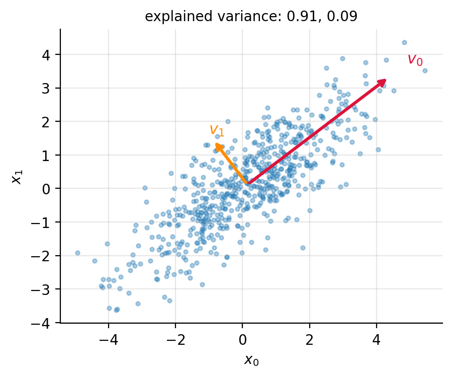
Figure 1.1: Six hundred samples from a Gaussian with covariance \(\bm{\Sigma}=\bigl(\begin{smallmatrix}3&2\\2&2\end{smallmatrix}\bigr)\), with the two eigenvectors of the sample covariance matrix drawn as arrows of length proportional to \(\sqrt{\lambda_i}\). The principal directions are orthogonal because \(\bm{\Sigma}\) is symmetric, Section The spectral decomposition of symmetric matrices.
1.10. The covariance matrix#
The single most important symmetric matrix in this book is built from the data themselves. Given \(n\) observations of \(p\) features collected in the design matrix \(\bm{X}\), write \(\bar{x}_j\) for the sample mean of column \(j\). The sample covariance between features \(j\) and \(k\) is
and these numbers assembled into a \(p\times p\) array form the covariance matrix \(\bm{\Sigma}\). For three features it reads
with the variances on the diagonal and the covariances off it. The divisor
\(n-1\) rather than \(n\) makes the estimate unbiased when the means have
themselves been estimated from the same data; it is what
numpy.cov uses, and the distinction matters only for small \(n\). A
fuller discussion belongs to Chapter 2; here we are
interested in \(\bm{\Sigma}\) as a matrix.
Covariance as a matrix product. Let \(\bm{X}_c\) denote the centred design matrix, obtained by subtracting from each column its mean. Then Eq. (1.57) is one entry of a matrix product and
This compact form tells us everything we need. The matrix is symmetric, since \((\bm{X}_c^{T}\bm{X}_c)^{T}=\bm{X}_c^{T}\bm{X}_c\); it is positive semi-definite, since \(\bm{z}^{T}\bm{X}_c^{T}\bm{X}_c\bm{z}=\|\bm{X}_c\bm{z}\|_2^2\ge0\) for every \(\bm{z}\); and by Section The spectral decomposition of symmetric matrices it therefore has real non-negative eigenvalues and an orthonormal eigenbasis. It is singular exactly when some linear combination of the centred features vanishes identically, which is to say when the features are exactly collinear, and it is nearly singular when they are nearly collinear. Note also that \(\bm{\Sigma}\) differs from \(\bm{X}^{T}\bm{X}\) of the normal equations (1.39) only by the centring and the factor \(1/(n-1)\): the matrix that governs the accuracy of a regression fit and the matrix that describes the spread of the data are, up to bookkeeping, the same object.
The companion matrix \(\bm{X}_c\bm{X}_c^{T}\), of size \(n\times n\), contains the inner products between observations rather than between features. It is the Gram matrix, and when the inner product is replaced by a kernel function it becomes the kernel matrix on which support vector machines and Gaussian processes are built. Sections The singular value decomposition and Principal component analysis will show that these two matrices carry exactly the same spectral information, which is why one may always work with whichever of \(p\) and \(n\) is smaller.
Correlation and whitening. Dividing each covariance by the two corresponding standard deviations gives the correlation matrix, \(\rho_{jk}=\sigma_{jk}/\sqrt{\sigma_{jj}\sigma_{kk}}\), with unit diagonal and entries in \([-1,1]\). Correlation is covariance made scale-free, and it is what one should inspect when features are measured in different units. Going further, the transformation
produces data whose covariance matrix is the identity: uncorrelated features of unit variance. This is whitening, and by Eq. (1.56) it is computed from the spectral decomposition of \(\bm{\Sigma}\). It is also where near-collinearity takes its revenge, since \(\bm{\Sigma}^{-1/2}\) divides by \(\sqrt{\lambda_i}\) and a tiny eigenvalue amplifies whatever noise happens to lie along that direction. Section Rank, the pseudoinverse and ill-conditioned design matrices explains what to do instead.
The following code constructs three correlated variables and extracts the spectrum of their covariance matrix.
import numpy as np

n = 100
x = np.random.normal(size=n)
y = 4.0 + 3.0 * x + np.random.normal(size=n)      # strongly correlated with x
z = x**3 + np.random.normal(size=n)

# np.cov expects variables in rows, so stack the three vectors vertically
W = np.vstack((x, y, z))
Sigma = np.cov(W)                                 # 3 x 3 covariance matrix
print(Sigma)

eigvals, eigvecs = np.linalg.eigh(Sigma)          # eigh: symmetric matrices
print(eigvals)
print(eigvals / np.sum(eigvals))                  # fraction of variance each
Note the use of np.linalg.eigh rather than np.linalg.eig.
The former exploits symmetry, returns real eigenvalues in ascending order and
guarantees orthonormal eigenvectors; the latter treats the matrix as general,
does none of these things, and is both slower and less accurate. Whenever a
matrix is known to be symmetric, say so.
Machine learning connection
The eigenvalues printed by the code above are the variances along the principal directions, and their ratios are what a scree plot displays. When one eigenvalue is very much smaller than the others, the data lie close to a lower-dimensional subspace: there are fewer genuinely independent features than columns. That single observation is the common root of dimensionality reduction, of multicollinearity in regression, and of the regularisation methods introduced to control it.
1.11. From algebra to computation#
Everything said so far is exact algebra. The moment we hand a matrix to a computer, however, two new questions arise. The first is one of accuracy: floating-point numbers carry a finite number of digits, and we need a way of measuring how large the resulting error is. The second is one of cost: a design matrix may have \(10^{6}\) rows, or a kernel matrix \(10^{5}\) rows and as many columns, and an algorithm whose work grows as \(n^3\) is then simply not available to us.
These two questions are not academic in machine learning; they are the subject. A regression problem whose features are nearly collinear will produce parameter estimates that swing wildly under a perturbation of the data too small to see, and no amount of statistical sophistication will repair that – it is a property of the matrix. A method that requires the factorisation of an \(n\times n\) matrix is unusable on a data set with a million observations, however elegant its derivation.
The remainder of this chapter is devoted to these two questions. We first
introduce the norms with which errors are measured and the condition number
that quantifies sensitivity, then develop the direct (elimination) methods for
linear systems, their iterative alternatives, and the algorithms for the
eigenvalue problem. We close with the singular value decomposition, which
answers simultaneously the questions of rank, of least squares, of compression
and of principal components. All programs are written in Python; the
complete, runnable versions are collected in the BookPrograms
directory.
Throughout we keep the convention of Section Notation and conventions that indices run from \(0\) to \(n-1\), so that the mathematical formulae and the Python code carry the same indices.
1.12. Vector and matrix norms#
A class of vector norms is given by the so-called \(p\)-norms
The three cases we shall need are \(p=1\), \(p=2\) and the limit \(p\rightarrow\infty\),
The \(2\)-norm is the one we have been using implicitly: it is the square root of the inner product of Section Vectors, and it is the ordinary Euclidean length.
These are not merely three ways of measuring the same thing. Applied to the residual \(\bm{y}-\bm{X}\bm{\theta}\), the choice of norm is the choice of loss function: minimising the \(2\)-norm gives ordinary least squares, which is the maximum-likelihood estimate under Gaussian noise and which weights large residuals heavily; minimising the \(1\)-norm gives least absolute deviations, which is far less sensitive to outliers; minimising the \(\infty\)-norm gives the minimax fit, which cares only about the single worst point. Applied instead to the parameter vector \(\bm{\theta}\) as a penalty, the same three norms give Ridge regression (\(\|\bm{\theta}\|_2^2\)), the Lasso (\(\|\bm{\theta}\|_1\)) and a rarely used minimax regularisation. The difference between Ridge and the Lasso – that the Lasso sets coefficients exactly to zero and Ridge merely shrinks them – is entirely a statement about the geometry of the unit balls of the two norms, as we show in Chapter 3.
Two inequalities follow from the definitions and will be used repeatedly. The first is the Cauchy-Schwarz inequality, valid for any two vectors in an inner product space,
with equality only when \(\bm{x}\) and \(\bm{y}\) are linearly dependent. Divided through by the two norms it states that a correlation coefficient can never exceed unity in magnitude. The second is the triangle inequality
which follows from Eq. (1.64). Proofs may be found in Golub and Van Loan [golub1996].
For matrices the most frequently used norms are the Frobenius norm
which is simply the \(2\)-norm of the matrix read as a long vector, and the induced or operator \(p\)-norms
The induced norm measures the largest factor by which \(\bm{A}\) can stretch a vector. For a symmetric matrix \(\|\bm{A}\|_2\) is the largest absolute eigenvalue, a fact which follows immediately from the spectral decomposition of Section The spectral decomposition of symmetric matrices. An orthogonal matrix has \(\|\bm{Q}\|_2=1\); it rotates but never stretches, which is Section Orthogonal transformations restated in the language of norms.
1.12.1. The Frobenius norm as a trace#
Definition (1.66) is a double sum over entries, which is convenient for a computer and inconvenient for a proof. The identity that makes the Frobenius norm usable in analysis is
for a real \(\bm{A}\), with \(\bm{A}^{T}\) replaced by \(\bm{A}^{\dagger}\) in the complex case. We give two proofs. The first is a line of index bookkeeping; the second explains why the identity has to hold, and it is the one worth remembering.
First proof: component by component. The product \(\bm{A}^{T}\bm{A}\) has entries
so that on the diagonal, where \(k=j\),
which is the squared Euclidean length of column \(j\) of \(\bm{A}\). The trace is the sum of the diagonal entries, so
the last step being nothing more than an interchange of two finite sums. The right-hand side is \(\|\bm{A}\|_F^2\) by definition, which proves Eq. (1.68). Read the calculation once more and it says something slightly stronger: the Frobenius norm squared is the sum of the squared column lengths, and by running the same argument on \(\bm{A}\bm{A}^{T}\) it is equally the sum of the squared row lengths. Hence \(\mathrm{Tr}(\bm{A}^{T}\bm{A})=\mathrm{Tr}(\bm{A}\bm{A}^{T})\) even though the two matrices have different dimensions.
The Frobenius inner product. The second proof begins by noticing that Eq. (1.68) is the norm statement of an inner product. For two matrices \(\bm{A},\bm{B}\) of the same shape define
where the second equality follows by repeating Eq. (1.69) with \(b_{ik}\) in place of \(a_{ik}\) and taking the trace. This is bilinear, symmetric, and positive definite – \(\langle\bm{A},\bm{A}\rangle_F\) is a sum of squares and vanishes only when every entry vanishes – so it is an inner product on the vector space of \(n\times p\) matrices, the Frobenius or Hilbert-Schmidt inner product. Every inner product induces a norm through \(\|\bm{A}\|=\sqrt{\langle\bm{A},\bm{A}\rangle}\), and for Eq. (1.70) that induced norm is precisely Eq. (1.66). Equation (1.68) is therefore not a coincidence about traces but the statement that the Frobenius norm is the norm belonging to the trace inner product.
Second proof: vectorisation. The same point can be made constructively. Let \(\mathrm{vec}(\bm{A})\) stack the columns of a matrix into one long vector,
The particular ordering is irrelevant for what follows; all that matters is that every entry appears exactly once. Then
by inspection, while for any two matrices of the same shape
using Eq. (1.70). Setting \(\bm{B}=\bm{A}\) gives Eq. (1.68) again. Geometrically, vectorisation is an isometry between matrix space equipped with the Frobenius norm and \(\mathbb{R}^{np}\) equipped with the ordinary Euclidean norm,
so \(\mathrm{Tr}(\bm{A}^{T}\bm{A})\) is simply the squared length of the matrix regarded as a point in \(np\) dimensions. Matrix space is a Euclidean space, and the Frobenius norm is what makes it one. Vectorisation is not only a proof device: it is what a deep learning framework does when it flattens the weights of a network into a single parameter vector for the optimiser.
Two consequences we shall use. First, the Frobenius norm is invariant under orthogonal transformations. If \(\bm{U}\) and \(\bm{V}\) are orthogonal of the appropriate sizes, then by the cyclic property of the trace
Choosing \(\bm{U}\) and \(\bm{V}\) to be the singular vectors of Section The singular value decomposition turns \(\bm{A}\) into its diagonal matrix of singular values, so
the Frobenius norm is the \(2\)-norm of the vector of singular values, and the Eckart-Young theorem of Section Low-rank approximation – that truncating the SVD gives the best low-rank approximation in the Frobenius norm – becomes a statement about discarding the smallest entries of that vector.
Second, because the Frobenius norm comes from an inner product, minimising it subject to linear constraints is an ordinary least-squares problem. This is what turns matrix factorisation into a tractable optimisation: the recommender-system objective \(\|\bm{R}-\bm{W}\bm{H}\|_F^2\), the non-negative matrix factorisation objective, and the secant-condition derivation of the BFGS update in the chapter on optimisation are all Frobenius-norm minimisations. The trace identity (1.68) is what makes the derivative \(\partial\,\mathrm{Tr}(\bm{X}^{T}\bm{X})/\partial\bm{X}=2\bm{X}\) of Eq. (1.47) available, and that single derivative is the whole of the derivation.
Relative error. Let \(fl(\bm{x})\) denote the machine representation of a vector \(\bm{x}\ne 0\). The relative error is
and if we use the \(\infty\)-norm the statement \(\|fl(\bm{x})-\bm{x}\|_{\infty}/\|\bm{x}\|_{\infty}\approx 10^{-l}\) says that the largest component of \(fl(\bm{x})\) carries roughly \(l\) correct significant digits. In IEEE double precision the machine epsilon is \(\varepsilon\approx2.2\times10^{-16}\), so about sixteen significant decimal digits are available before any computation has been performed.
The condition number.
Suppose we solve \(\bm{A}\bm{x}=\bm{b}\) but, because of rounding, actually solve a slightly perturbed problem with right-hand side \(\bm{b}+\delta\bm{b}\). The resulting error \(\delta\bm{x}\) satisfies \(\bm{A}\,\delta\bm{x}=\delta\bm{b}\), hence \(\|\delta\bm{x}\|\le\|\bm{A}^{-1}\|\,\|\delta\bm{b}\|\), while \(\|\bm{b}\|\le\|\bm{A}\|\,\|\bm{x}\|\). Combining the two gives
The quantity \(\kappa(\bm{A})\) is the condition number. It tells us how much an input error can be amplified, and it is a property of the problem, not of the algorithm: no amount of cleverness can rescue an ill-conditioned system. In the \(2\)-norm and for a symmetric matrix
so a matrix is ill-conditioned exactly when it has eigenvalues of very different magnitude, that is, when it is close to being singular. As a rule of thumb, if \(\kappa\approx 10^{k}\) one loses about \(k\) significant digits.
Figure 1.2 makes the point concrete for the polynomial design matrix we shall fit in Chapter 3. The condition number of \(\bm{X}\) itself grows exponentially with the degree, and that of \(\bm{X}^{T}\bm{X}\) grows as its square, so that by degree eight the normal equations already have a condition number exceeding \(1/\varepsilon_{\mathrm{mach}}\) – at which point double precision retains no correct digits at all. Nothing is wrong with the mathematics; the difficulty is entirely one of representation, and it is the reason the least-squares routines of Chapter 3 avoid forming the product.
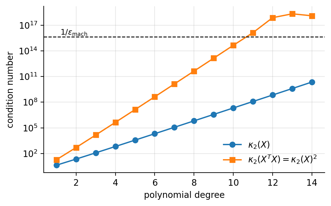
Figure 1.2: Condition number of the Vandermonde matrix of a polynomial fit to \(100\) points on \([0,1]\), against the polynomial degree. Squaring the matrix squares the condition number, Eq. (1.118); the dashed line marks the reciprocal of the machine epsilon, beyond which no significant digits survive.
Machine learning connection
Ill-conditioning is the numerical name for multicollinearity. If two features are strongly correlated, the matrix \(\bm{X}^{T}\bm{X}\) of the normal equations (1.39) has a small eigenvalue, its condition number is large, and the fitted coefficients become enormous and of opposite sign – the model compensates one feature against the other, and a change in the data too small to notice moves the coefficients by a great deal. Two remarks follow. First, the damage is done before any statistics is involved; it is visible in \(\kappa_2(\bm{X})\) alone. Second, Eq. (1.42) shows what the Ridge penalty does about it: adding \(\lambda\) to every eigenvalue changes the condition number from \(\lambda_{\max}/\lambda_{\min}\) to \((\lambda_{\max}+\lambda)/(\lambda_{\min}+\lambda)\), which is smaller for every \(\lambda>0\). Regularisation is, among other things, a numerical conditioning device.
1.13. Linear systems and Gaussian elimination#
We now turn to the solution of
with \(\bm{A}\) square and non-singular. Before describing the algorithms it is worth recalling why such systems appear at all.
Where linear systems come from. The example that matters most in this book has already been derived. Setting the gradient (1.38) of the least-squares cost to zero produced the normal equations
which is Eq. (1.78) with \(\bm{A}=\bm{X}^{T}\bm{X}\) of size \(p\times p\) and \(\bm{w}=\bm{X}^{T}\bm{y}\). Fitting a linear model is solving a linear system, and the properties of that system – its size, its symmetry, its conditioning – decide which of the algorithms below is appropriate. The same structure recurs throughout: the interpolation coefficients of a spline, the dual coefficients of a kernel ridge regression, the Newton step of an optimisation method and the update of a Gaussian process posterior are all solutions of a linear system with a symmetric positive definite matrix.
The elimination. The idea of Gaussian elimination is to use the first equation to eliminate \(x_0\) from the remaining \(n-1\) equations, then the new second equation to eliminate \(x_1\) from the remaining \(n-2\), and so on. After \(n-1\) such steps we are left with an upper triangular system
which is solved from the bottom upwards by backward substitution
To eliminate \(x_0\) we multiply the first equation by \(a_{j0}/a_{00}\) and subtract it from equation \(j\), for \(j=1,\dots,n-1\). The elements of the remaining \((n-1)\times(n-1)\) block are updated according to
and the same formula, applied to successively smaller blocks, defines the whole algorithm. Counting operations, the elimination requires \(2n^3/3+\bigO(n^2)\) floating point operations, while the backward substitution costs only \(\bigO(n^2)\). The elimination dominates, and this cubic scaling is the reason direct methods become unusable for the large problems of Section Iterative methods for linear systems.
Pivoting.
The derivation assumed \(a_{00}\ne0\), and more generally that no pivot element vanishes. Even a small pivot is dangerous, since dividing by it amplifies rounding errors. Suppose the first division produces \(-10^{-7}\) where the original entry was of order one: we are then adding \(10^{7}+1\), and in single precision the result is \(10^{7}\). The information carried by the small entry has been destroyed. The cure is partial pivoting: before eliminating column \(k\) we search the column for the element of largest absolute value and interchange rows so that this element becomes the pivot. Row interchanges do not alter the solution, and they keep all multipliers bounded by unity. In practice one always pivots.
The following class implements the algorithm.
class GaussianElimination(DirectSolver):
    """Gaussian elimination with partial pivoting."""

    def solve(self, b):
        n = self.n
        M = self.A.copy()                 # the elimination destroys its input
        y = np.asarray(b, dtype=float).copy()

        for k in range(n - 1):            # forward elimination
            # partial pivoting: use the largest element in the column
            p = k + np.argmax(np.abs(M[k:, k]))
            if abs(M[p, k]) < 1.0e-14:
                raise np.linalg.LinAlgError("matrix is singular")
            if p != k:
                M[[k, p]] = M[[p, k]]
                y[k], y[p] = y[p], y[k]
            for i in range(k + 1, n):
                factor = M[i, k] / M[k, k]
                M[i, k:] -= factor * M[k, k:]
                y[i] -= factor * y[k]

        return self._back_substitute(M, y)

    @staticmethod
    def _back_substitute(U, y):
        """Solve U x = y for an upper triangular U."""
        n = U.shape[0]
        x = np.zeros(n)
        for m in range(n - 1, -1, -1):
            x[m] = (y[m] - U[m, m+1:] @ x[m+1:]) / U[m, m]
        return x
1.14. LU and Cholesky decompositions#
Gaussian elimination as written above throws away the multipliers once it has used them. If we keep them instead, we obtain a factorisation of \(\bm{A}\) itself, and this is what makes the method reusable. The LU decomposition writes
with \(\bm{L}\) unit lower triangular and \(\bm{U}\) upper triangular; for a \(4\times 4\) matrix
The factorisation exists whenever \(\bm{A}\) is non-singular and, with the normalisation \(l_{ii}=1\), it is unique. Multiplying out the first column gives \(a_{00}=u_{00}\) and \(a_{j0}=l_{j0}u_{00}\), which determines \(u_{00}\) and the multipliers \(l_{j0}\). The second column then gives \(u_{01}\), \(u_{11}\) and \(l_{j1}\), and so on: at every stage the unknowns are determined by quantities already computed. In practice \(\bm{L}\) and \(\bm{U}\) are stored in the same array as \(\bm{A}\), since the unit diagonal of \(\bm{L}\) need not be kept.
With partial pivoting the factorisation reads \(\bm{P}\bm{A}=\bm{L}\bm{U}\) with \(\bm{P}\) a permutation matrix, which in the program is recorded as a permutation array rather than as a matrix.
The determinant. Because \(\det(\bm{L})=1\) and the determinant of a triangular matrix is the product of its diagonal elements,
where the sign is \((-1)^{r}\) with \(r\) the number of row interchanges. This is the only sensible way of computing a determinant numerically; expanding in minors would cost \(\bigO(n!)\) operations.
Solving the system. Writing \(\bm{A}\bm{x}=\bm{L}\bm{U}\bm{x}=\bm{w}\) and introducing the intermediate vector \(\bm{y}=\bm{U}\bm{x}\), the problem splits into two triangular systems,
each costing only \(\bigO(n^2)\) operations. This is the decisive advantage of LU over plain elimination: the expensive \(\bigO(n^3)\) factorisation is performed once, after which any number of right-hand sides can be treated cheaply. In a cross-validation loop, or when refitting a model with several different targets on the same features, this is the difference between one factorisation and a dozen.
The inverse, and why not to compute it.
Column \(j\) of \(\bm{A}^{-1}\) is the solution of \(\bm{A}\bm{x}=\bm{e}_j\), where
\(\bm{e}_j\) is the \(j\)th unit vector. The inverse therefore costs one
factorisation plus \(n\) substitutions. It is worth stressing that one should
almost never compute an inverse: if the aim is to solve a linear system,
solving it directly is both faster and more accurate than forming
\(\bm{A}^{-1}\) and multiplying. The formula
\(\bm{\theta}=(\bm{X}^{T}\bm{X})^{-1}\bm{X}^{T}\bm{y}\) is a statement about
\(\bm{\theta}\), not an instruction to a computer; the instruction is
np.linalg.solve or, better still, np.linalg.lstsq.
class LUDecomposition(DirectSolver):
    """Doolittle LU factorisation with partial pivoting, P A = L U."""

    def _factorize(self):
        n = self.n
        LU = self.A.copy()
        perm = np.arange(n)
        sign = 1.0

        for k in range(n):
            p = k + np.argmax(np.abs(LU[k:, k]))
            if abs(LU[p, k]) < 1.0e-14:
                raise np.linalg.LinAlgError("matrix is singular")
            if p != k:
                LU[[k, p]] = LU[[p, k]]
                perm[[k, p]] = perm[[p, k]]
                sign = -sign
            # the multipliers l_ik are stored in place, below the diagonal
            LU[k+1:, k] /= LU[k, k]
            # rank-one update of the trailing submatrix
            LU[k+1:, k+1:] -= np.outer(LU[k+1:, k], LU[k, k+1:])

        self.LU, self.perm, self.sign = LU, perm, sign

    def solve(self, b):
        """Solve A x = b in two steps: L y = P b, then U x = y."""
        y = np.asarray(b, dtype=float)[self.perm].copy()
        n = self.n
        for i in range(1, n):                    # forward, L has unit diagonal
            y[i] -= self.LU[i, :i] @ y[:i]
        x = np.zeros(n)
        for i in range(n - 1, -1, -1):           # backward
            x[i] = (y[i] - self.LU[i, i+1:] @ x[i+1:]) / self.LU[i, i]
        return x

    def determinant(self):
        return self.sign * np.prod(np.diag(self.LU))
Cholesky’s factorisation.
If \(\bm{A}\) is real, symmetric and positive definite it admits the special factorisation
with \(\bm{L}\) lower triangular. The elements follow from
The algorithm costs half of a general LU factorisation, and since the pivots \(L_{ii}\) are guaranteed positive there is no need for pivoting at all. The square root in Eq. (1.87) also provides the cheapest available test of positive definiteness: if the argument turns negative, the matrix is not positive definite.
Machine learning connection
Cholesky is the workhorse of every method whose central object is a symmetric positive definite matrix, and there are many. The normal equations (1.39) have \(\bm{X}^{T}\bm{X}\) on the left, and their regularised form (1.42) guarantees positive definiteness for any \(\lambda>0\); Gaussian process regression requires the solution of \((\bm{K}+\sigma^2\bm{I})\bm{\alpha}=\bm{y}\) with \(\bm{K}\) a kernel matrix, and its log-marginal-likelihood needs \(\ln\Det{K+\sigma^2 I}\), which Eq. (1.84) reads off the Cholesky factor as \(2\sum_i\ln L_{ii}\); and sampling from a multivariate Gaussian with covariance \(\bm{\Sigma}\) is done by drawing \(\bm{z}\sim N(\bm{0},\bm{I})\) and forming \(\bm{L}\bm{z}\). When a Cholesky factorisation fails in a Gaussian process code, the message is not that the linear algebra is broken but that the kernel matrix has lost positive definiteness to rounding, and the standard remedy – adding a small multiple of the identity, the “jitter” – is Eq. (1.42) under another name.
1.15. Iterative methods for linear systems#
The methods of the previous sections are direct: up to rounding they produce the exact answer in a finite, known number of operations. Their cost, however, grows as \(n^3\), and they require the matrix to be stored. Iterative methods take the opposite view. We start from a guess and improve it until the change falls below a tolerance. The matrix enters only through the product \(\bm{A}\bm{x}\), so a matrix that is sparse, or that is never formed at all but only applied, costs nothing extra. This is the reason iterative methods, and not the direct ones, are what one uses for large-scale problems.
We split the matrix as
with \(\bm{D}\) diagonal, \(\bm{L}\) strictly lower and \(\bm{U}\) strictly upper triangular.
Jacobi’s method.
Solving row \(i\) for \(x_i\) and evaluating the right-hand side with the previous iterate gives
or, in matrix form,
Every component of the new iterate is computed from the old ones only, so all \(n\) updates are independent and the method parallelises trivially. It converges whenever \(\bm{A}\) is strictly diagonally dominant or symmetric positive definite.
Gauss-Seidel.
Nothing forces us to wait: the components \(x_0^{(k+1)},\dots,x_{i-1}^{(k+1)}\) are already available when we compute \(x_i^{(k+1)}\). Using them immediately gives the Gauss-Seidel iteration
This is forward substitution applied to the splitting, and it typically halves the number of iterations. The price is that the sweep is now inherently sequential. Readers who have met coordinate descent for the Lasso will recognise the pattern: update one coordinate at a time, using the most recent values of all the others.
Successive over-relaxation.
Gauss-Seidel usually moves in the right direction but not far enough. Over-relaxation exaggerates the step by a factor \(\omega\),
which in matrix form reads
For symmetric positive definite matrices convergence is guaranteed for \(0<\omega<2\), and \(\omega=1\) returns Gauss-Seidel. A well chosen \(\omega\) can reduce the iteration count by an order of magnitude, but the optimal value depends on the spectrum of \(\bm{A}\) and is rarely known in advance – an early instance of the hyperparameter problem that pervades this book.
1.16. The conjugate gradient method#
The methods above treat the linear system as a fixed-point problem. The conjugate gradient method instead treats it as a minimisation, which puts it in the same family as the optimisation algorithms of the chapter on optimisation. For a symmetric positive definite \(\bm{A}\) the solution of \(\bm{A}\bm{x}=\bm{b}\) is the unique minimum of the quadratic form
since by Eqs. (1.25) and (1.27) \(\nabla P = \bm{A}\bm{x}-\bm{b}\), which vanishes precisely at the solution. Taking \(\bm{A}=\bm{X}^{T}\bm{X}\) and \(\bm{b}=\bm{X}^{T}\bm{y}\) recovers the least-squares problem, so what follows is a solver for linear regression as much as for a linear system. The residual
is the negative gradient of \(P\), and steepest descent would move along it. Steepest descent is however notoriously slow, because successive steps undo part of the progress of their predecessors; the number of iterations grows with the condition number of \(\bm{A}\), which for the normal equations is the square of that of \(\bm{X}\).
The remedy is to search along directions that are conjugate, meaning orthogonal with respect to the inner product defined by \(\bm{A}\),
The eigenvectors of \(\bm{A}\) are an example, since \(\bm{v}_i^{T}\bm{A}\bm{v}_j=\lambda_j\bm{v}_i^{T}\bm{v}_j\) vanishes for \(i\neq j\); but the whole point of the method is that we shall construct conjugate directions without knowing any eigenvectors. A set of \(n\) mutually conjugate vectors forms a basis, so we may expand
Multiplying \(\bm{A}\bm{x}=\bm{b}\) from the left by \(\bm{p}_k^{T}\) and using Eq. (1.97) collapses the sum to a single term,
so each direction can be treated independently. In exact arithmetic the method therefore terminates after at most \(n\) steps, which makes it a direct method in disguise; what makes it useful is that a good approximation is normally reached in far fewer. The directions are generated on the fly: starting from \(\bm{x}_0=\bm{0}\) and \(\bm{p}_0=\bm{r}_0=\bm{b}\), the new direction is the residual with its component along the previous direction projected out,
which is one step of Gram-Schmidt, Eq. (1.11), performed in the inner product defined by \(\bm{A}\). Remarkably, the new direction is automatically conjugate to all previous ones, not merely the last, so the recursion needs to store only a handful of vectors.
def conjugate_gradient(A, b, x0=None, tol=1.0e-10, maxiter=None):
    """Solve A x = b for symmetric positive definite A.

    A may be a matrix or any callable implementing the product A @ v,
    which is what makes the method usable when A is never formed.
    """
    matvec = A if callable(A) else (lambda v: A @ v)
    n = b.shape[0]
    x = np.zeros(n) if x0 is None else np.asarray(x0, dtype=float).copy()

    r = b - matvec(x)
    p = r.copy()
    rsold = r @ r

    for _ in range(maxiter or n):
        Ap = matvec(p)
        alpha = rsold / (p @ Ap)
        x += alpha * p
        r -= alpha * Ap
        rsnew = r @ r
        if np.sqrt(rsnew) < tol:
            break
        p = r + (rsnew / rsold) * p        # Fletcher-Reeves update
        rsold = rsnew

    return x
Note the signature. The matrix is accepted either as an array or as a
function computing \(\bm{A}\bm{v}\), and for the normal equations that function
is lambda v: X.T @ (X @ v), which never forms the \(p\times p\) product
\(\bm{X}^{T}\bm{X}\) at all. For a design matrix with many features this is the
difference between a feasible computation and an impossible one, and it is the
same matrix-free idea that makes stochastic gradient descent practical.
Machine learning connection
The convergence of conjugate gradient is governed by \(\sqrt{\kappa_2(\bm{A})}\), whereas that of steepest descent is governed by \(\kappa_2(\bm{A})\) itself; the square root is the whole advantage. Since \(\kappa_2(\bm{X}^{T}\bm{X})=\kappa_2(\bm{X})^2\), applying conjugate gradient to the normal equations restores exactly the conditioning one loses by forming them. Preconditioning – solving \(\bm{M}^{-1}\bm{A}\bm{x} = \bm{M}^{-1}\bm{b}\) for some cheaply invertible \(\bm{M}\) that approximates \(\bm{A}\) – pushes this further, and the simplest choice, \(\bm{M}=\bm{D}\), amounts to rescaling each feature by its standard deviation. Feature standardisation, which we introduced in Section Arrays in practice: numpy, BLAS and LAPACK as a statistical convention, is also a preconditioner.
1.17. The algebraic eigenvalue problem#
We return to the eigenvalue problem of Section The spectral decomposition of symmetric matrices, this time asking how it is actually solved. The eigenvalues of a matrix \(\bm{A}\) of dimension \(n\) are defined by
where, unless stated otherwise, eigenvector means right eigenvector. Rewriting Eq. (1.101) as \((\bm{A}-\lambda^{(\nu)}\bm{I})\bm{x}^{(\nu)}=\bm{0}\), a non-trivial solution exists only if the matrix is singular, that is only if the characteristic polynomial
vanishes. Its roots form the spectrum \(\lambda(\bm{A})\), and the factorisation gives back Eq. (1.55).
It is tempting to conclude that one should find eigenvalues by computing the characteristic polynomial and looking for its roots. This is almost always a bad idea: the roots of a polynomial are extremely sensitive to its coefficients, so the detour through \(P(\lambda)\) throws away accuracy that the original matrix still contained. The standard approach is entirely different. We apply a sequence of similarity transformations that bring \(\bm{A}\) towards diagonal form.
1.17.1. Similarity transformations#
Let \(\bm{A}\) be real and symmetric. Then there exists a real orthogonal matrix \(\bm{S}\) such that
and the \(j\)th column of \(\bm{S}\) is the eigenvector belonging to \(\lambda_j\) [golub1996]. More generally, \(\bm{B}\) is a similarity transform of \(\bm{A}\) if
The importance of such a transformation is that it leaves the eigenvalues unchanged while altering the eigenvectors in a controlled way. The proof is one line. Multiply \(\bm{A}\bm{x}=\lambda\bm{x}\) from the left by \(\bm{S}^{T}\) and insert \(\bm{S}\bm{S}^{T}=\bm{I}\) between \(\bm{A}\) and \(\bm{x}\),
that is \(\bm{B}(\bm{S}^{T}\bm{x})=\lambda(\bm{S}^{T}\bm{x})\). So \(\lambda\) is an eigenvalue of \(\bm{B}\) as well, with eigenvector \(\bm{S}^{T}\bm{x}\). The strategy is therefore to apply transformations until
1.17.2. The power method#
The simplest of all eigenvalue algorithms is worth understanding, because much of what a library routine does can be seen as a refinement of it, and because it reappears in its own right in the analysis of Markov chains and of network centrality. Assume \(\bm{A}\) can be diagonalised, with eigenvalues \(\lambda_0,\dots,\lambda_{n-1}\) and eigenvectors \(\bm{v}_0,\dots,\bm{v}_{n-1}\), and assume there is a dominant eigenvalue, \(|\lambda_0|>|\lambda_j|\) for \(j>0\). An arbitrary starting vector expands as
and applying \(\bm{A}\) repeatedly gives
Every ratio \(|\lambda_j/\lambda_0|\) is smaller than one, so the bracket tends to \(\bm{v}_0\): repeated multiplication filters out everything except the dominant eigenvector. Normalising at every step, \(\bm{b}_{k}=\bm{A}^{k}\bm{b}_0/\|\bm{A}^{k}\bm{b}_0\|\), and estimating the eigenvalue by the Rayleigh quotient
we obtain a method that converges geometrically with ratio \(|\lambda_1/\lambda_0|\). When the two largest eigenvalues are close, convergence is correspondingly slow.
The power method has two obvious weaknesses: it gives only one eigenpair, and
it discards the information contained in the intermediate vectors
\(\bm{b}_0,\bm{A}\bm{b}_0,\dots,\bm{A}^{k-1}\bm{b}_0\). Removing the second
weakness by working in the whole space spanned by those vectors, the
Krylov space, leads to the Lanczos and Arnoldi algorithms, which is
how scipy.sparse.linalg.eigsh computes a few extreme eigenpairs of a
large sparse matrix without ever factorising it. Applying the power method to
\(\bm{A}^{-1}\) instead gives inverse iteration, which converges to the
eigenvalue of smallest magnitude and, with a shift, to any eigenvalue one can
bracket.
Machine learning connection
Equation (1.108) is the PageRank algorithm. The importance vector of a set of web pages is the dominant eigenvector of a stochastic link matrix, and it is computed by precisely the iteration above – multiply, normalise, repeat – on a matrix far too large to factorise. The same iteration, applied to the covariance matrix, gives the first principal component, and applied to \(\bm{X}^{T}\bm{X}\) implicitly through two matrix-vector products it gives the first singular vector of \(\bm{X}\) without forming any product at all.
1.17.3. What library routines actually do#
The algorithms used in practice reduce the matrix to a simpler form by orthogonal similarity transformations before extracting eigenvalues. For a symmetric matrix, a finite sequence of Householder reflections,
each of which zeroes all but one entry of a column below the diagonal, brings
\(\bm{A}\) to tridiagonal form in \(\bigO(n^3)\) operations; an iterative QR or QL
sweep with shifts then drives the off-diagonal elements to zero, and converges
cubically. This two-stage strategy – a finite orthogonal reduction followed
by an iterative sweep on the reduced matrix – is what LAPACK implements and
what numpy.linalg.eigh calls. Jacobi’s method of successive plane
rotations, which attacks the full matrix directly, is the historically older
alternative and remains attractive on parallel hardware.
We shall use the library routines throughout. It is worth knowing what they do, and worth knowing that they cost \(\bigO(n^3)\): an eigendecomposition of a \(10^4\times10^4\) covariance matrix is a serious computation, and one of a \(10^6\times10^6\) kernel matrix is not a computation at all. The remedies are the Krylov methods mentioned above, randomised algorithms, and the observation of Section Principal component analysis that one rarely needs the whole spectrum.
1.18. The singular value decomposition#
Every algorithm so far has assumed a square matrix, and most of them a symmetric one. The design matrix of Eq. (1.1) is neither. It has \(n\) rows and \(p\) columns, and there is no reason whatever for those two numbers to agree. For rectangular matrices we need a decomposition that does not require squareness, and preferably one that does not require diagonalisability either.
Recall that a square matrix can be diagonalised if and only if it is normal, that is if \(\bm{X}\bm{X}^{T}=\bm{X}^{T}\bm{X}\). Not every matrix satisfies this. The simplest counterexample is
whose determinant vanishes and for which \(\bm{X}\bm{X}^{T}\neq\bm{X}^{T}\bm{X}\). It is defective: it cannot be diagonalised, and it has no inverse. A data set with two perfectly anticorrelated features produces exactly this matrix, so the case is not pathological but routine.
The singular value decomposition has no such restriction.
The theorem. Any \(n\times p\) matrix \(\bm{X}\), real or complex, square or rectangular, can be written
where \(\bm{U}\) is an \(n\times n\) orthogonal matrix, \(\bm{U}\bm{U}^{T}=\bm{U}^{T}\bm{U}=\bm{I}_n\), where \(\bm{V}\) is a \(p\times p\) orthogonal matrix, \(\bm{V}\bm{V}^{T}=\bm{V}^{T}\bm{V}=\bm{I}_p\), and where \(\bm{\Sigma}\) is an \(n\times p\) matrix which is zero except on the main diagonal, on which sit the singular values
The columns of \(\bm{U}\) are the left singular vectors and the columns of \(\bm{V}\) the right singular vectors. The decomposition always exists. For the defective matrix of Eq. (1.111) it reads
with \(\sigma_0=2\) and \(\sigma_1=0\). A matrix that cannot be diagonalised at all is decomposed without difficulty, and the vanishing singular value states plainly what the determinant only hinted at: the two columns carry one direction of information between them.
Geometry. Equation (1.112) says that every linear map is a rotation, followed by a scaling along the new axes, followed by another rotation. The singular values are the scale factors, and \(\|\bm{X}\|_2=\sigma_0\), which is the statement of Section Vector and matrix norms that the induced \(2\)-norm measures the largest stretching a matrix can produce. For a design matrix the picture is concrete: the right singular vectors are directions in feature space, the left singular vectors are patterns across observations, and the singular values say how much of the data lies along each such pairing.
Relation to the eigenvalue problem. The SVD is not an independent construction; it is the symmetric eigenvalue problem of Section The algebraic eigenvalue problem in disguise. Using Eq. (1.112) and the orthogonality of \(\bm{U}\),
where \(\tilde{\bm{\Sigma}}\) is the \(p\times p\) diagonal matrix of singular values. Multiplying from the right by \(\bm{V}\) gives
so the right singular vectors are the eigenvectors of \(\bm{X}^{T}\bm{X}\) and the squared singular values its eigenvalues. In exactly the same way
with the remaining \(n-r\) eigenvalues equal to zero. Every singular value is therefore the non-negative square root of an eigenvalue of \(\bm{X}^{T}\bm{X}\), and if \(\bm{X}\) is itself symmetric the singular values are the absolute values of its eigenvalues.
These two relations do a great deal of work in what follows. Read together with Section The covariance matrix they say that the covariance matrix \(\bm{X}_c^{T}\bm{X}_c/(n-1)\) and the Gram matrix \(\bm{X}_c\bm{X}_c^{T}\) share their non-zero spectrum entirely: the eigenvalues of the \(p\times p\) matrix and of the \(n\times n\) one are the same numbers, up to zeros. One may therefore always work with whichever is smaller, which is what makes principal component analysis feasible both when \(p\gg n\) and when \(n\gg p\).
The economy-size decomposition.
If \(n>p\) the last \(n-p\) columns of \(\bm{U}\) are multiplied by zeros in
\(\bm{\Sigma}\) and can never contribute. Removing them, and the corresponding
rows of zeros in \(\bm{\Sigma}\), gives the economy-size decomposition, in which
\(\bm{U}\) is \(n\times p\) and \(\bm{\Sigma}\) is \(p\times p\). If \(p>n\) one keeps
instead the first \(n\) columns of \(\bm{V}\). Nothing is lost and both storage
and work are reduced; this is full_matrices=False in numpy, and it
is what one should almost always ask for.
How not to compute it. Equation (1.116) suggests an algorithm: form \(\bm{X}^{T}\bm{X}\), diagonalise it with the machinery of Section What library routines actually do, take square roots. This is mathematically correct and numerically poor. From Eq. (1.77) the condition number of the product is the square of that of \(\bm{X}\),
so half of the available significant digits are destroyed before the eigenvalue solver is even called. Table 1.2 shows the damage for a \(60\times 12\) matrix constructed with singular values spread logarithmically between \(1\) and \(10^{-7}\): the direct SVD returns all twelve to machine precision, the detour through \(\bm{X}^{T}\bm{X}\) loses seven digits on the smallest.
Exact \(\sigma_i\) |
From the SVD |
From \(\bm{X}^{T}\bm{X}\) |
Relative error |
|---|---|---|---|
\(1.00000000\times10^{0}\) |
\(1.00000000\times10^{0}\) |
\(1.00000000\times10^{0}\) |
\(4.4\times10^{-16}\) |
\(6.57933225\times10^{-4}\) |
\(6.57933225\times10^{-4}\) |
\(6.57933225\times10^{-4}\) |
\(2.0\times10^{-11}\) |
\(1.87381742\times10^{-6}\) |
\(1.87381742\times10^{-6}\) |
\(1.87381889\times10^{-6}\) |
\(7.8\times10^{-7}\) |
\(4.32876128\times10^{-7}\) |
\(4.32876128\times10^{-7}\) |
\(4.32893930\times10^{-7}\) |
\(4.1\times10^{-5}\) |
\(1.00000000\times10^{-7}\) |
\(1.00000000\times10^{-7}\) |
\(9.99683051\times10^{-8}\) |
\(3.2\times10^{-4}\) |
Table 1.2: Singular values of a \(60\times12\) matrix with \(\kappa_2(\bm{X})=10^{7}\), computed directly and through the eigenvalues of \(\bm{X}^{T}\bm{X}\), for which \(\kappa_2=10^{14}\). Forming the product costs roughly half the significant digits.
The stable algorithm never forms the product. It reduces \(\bm{X}\) to
bidiagonal form by Householder reflectors, Eq. (1.110),
applied alternately from the left and the right, and then runs an implicitly
shifted QR sweep on the bidiagonal matrix. This is the Golub-Kahan algorithm,
and it is what numpy.linalg.svd calls through LAPACK.
Figure 1.3 shows the same comparison graphically. The singular values computed directly by the Golub-Kahan algorithm lie on the exact values over the whole range of thirteen orders of magnitude, while those obtained as square roots of the eigenvalues of \(\bm{X}^{T}\bm{X}\) peel away from the truth once \(\sigma_i\) falls below about \(\sqrt{\varepsilon}\sigma_0\). The failure is not gradual in any useful sense: precisely the small singular values, which are the ones we consult in order to detect near-collinearity, are the ones destroyed.
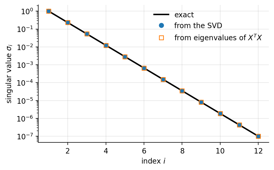
Figure 1.3: Singular values of a \(60\times12\) matrix constructed with \(\sigma_i\) spread logarithmically between \(1\) and \(10^{-7}\). The direct SVD reproduces all twelve; forming \(\bm{X}^{T}\bm{X}\) first loses the smallest, as anticipated by Table 1.2.
Machine learning connection
Equation (1.118) is the
reason that solving a regression problem through the normal
equations (1.39) is a poor idea whenever the features
are at all collinear. Forming \(\bm{X}^{T}\bm{X}\) squares the condition
number, so a design matrix with \(\kappa_2(\bm{X})=10^{8}\) – unremarkable for
a polynomial fit of modest degree – yields a system with \(\kappa_2=10^{16}\),
at which point double precision retains nothing. This is why
numpy.linalg.lstsq, and LinearRegression in
scikit-learn,
do not solve the normal equations at all. They use the SVD, or a QR
decomposition, and work with \(\kappa_2(\bm{X})\) throughout. We write the
normal equations because they are how one derives the estimator; we
compute with the SVD because it is how one evaluates it.
1.19. Rank, the pseudoinverse and ill-conditioned design matrices#
The rank of a matrix is the number of linearly independent columns, and the SVD reads it off immediately: it is the number of non-zero singular values. In floating-point arithmetic one asks instead for the numerical rank, the number of singular values above a threshold, typically \(\max(n,p)\,\varepsilon\,\sigma_0\) with \(\varepsilon\) the machine precision. A design matrix is rank deficient when some feature is an exact linear combination of others, and near rank deficient – which is the practically dangerous case – when it nearly is. The condition number of Section Vector and matrix norms is likewise a statement about singular values,
which is infinite exactly when \(\bm{X}\) is singular. The SVD thus not only detects near-singularity, it quantifies it.
The Moore-Penrose pseudoinverse. When \(\bm{X}^{-1}\) does not exist – and for a rectangular design matrix it never does – or exists but is useless because \(\bm{X}\) is nearly singular, the SVD provides the natural substitute
where \(\bm{\Sigma}^{+}\) is obtained from \(\bm{\Sigma}\) by transposing it and replacing every non-zero singular value by its reciprocal, leaving the zeros as zeros. In practice one treats as zero every singular value below some \(\varepsilon_{\mathrm{cut}}\sigma_0\). Inverting a singular value of \(10^{-13}\) would amplify the rounding noise in the corresponding direction by \(10^{13}\); discarding it simply declares that the data contain no information about that direction, which is the truth.
Least squares through the pseudoinverse. The pseudoinverse is not merely a formal device. Substituting the SVD into the normal equations (1.39) and using Eq. (1.115),
so the least-squares estimator is the pseudoinverse applied to the targets. Written componentwise this reads
which repays careful reading. The fit is a sum over directions in feature space. Each contributes the component of the target along the corresponding left singular vector, divided by the singular value. A direction along which the data barely vary has a small \(\sigma_i\), and dividing by it amplifies whatever noise happens to lie along \(\bm{u}_i\). This is multicollinearity, seen from the inside: it is not that the estimator is biased or that the statistics is wrong, it is that Eq. (1.122) divides by a small number. When the smallest singular values are dropped rather than inverted, the result is truncated SVD regression or principal component regression, and when they are damped rather than dropped, the result is Ridge regression – which is Section Ridge regression through the singular value decomposition.
Equation (1.122) also disposes of the case \(p>n\), more features than observations, in which \(\bm{X}^{T}\bm{X}\) is singular and the normal equations have infinitely many solutions. The pseudoinverse selects among them the solution of smallest \(2\)-norm, which is a perfectly definite and often sensible answer, and it does so without any special-case logic.
import numpy as np

def lstsq_svd(X, y, rcond=1.0e-12):
    """Least-squares fit through the SVD, with explicit truncation.

    Returns the coefficients, the singular values, and the numerical rank.
    """
    U, s, Vt = np.linalg.svd(X, full_matrices=False)
    keep = s > rcond * s[0]                 # numerical rank
    theta = (Vt[keep].T * (1.0 / s[keep])) @ (U[:, keep].T @ y)
    return theta, s, int(np.sum(keep))

# A deliberately collinear design matrix: the third column is nearly the
# sum of the first two.
rng = np.random.default_rng(2024)
n = 200
x1, x2 = rng.normal(size=n), rng.normal(size=n)
X = np.column_stack([x1, x2, x1 + x2 + 1.0e-6 * rng.normal(size=n)])
y = 1.0 + 2.0 * x1 - x2 + 0.1 * rng.normal(size=n)

theta, s, rank = lstsq_svd(X, y)
print("singular values:", s)
print("condition number:", s[0] / s[-1])
print("numerical rank:", rank)
The three singular values of this design matrix span some seven orders of magnitude, and the coefficients returned by an untruncated fit are enormous and mutually cancelling. Truncating the smallest singular value returns a rank-two fit whose predictions are essentially identical and whose coefficients are of order unity. Nothing has been lost: the third feature never carried independent information.
Machine learning connection
It is worth being explicit about what the truncation threshold buys. Keeping a direction with a tiny singular value adds a term to Eq. (1.122) with an enormous coefficient, which fits the noise in the training data and generalises catastrophically. Discarding it introduces a small bias and a large reduction in variance. The threshold is therefore not a numerical detail but a hyperparameter, chosen by the same cross-validation that chooses \(\lambda\) in Ridge regression, and the bias-variance trade-off of Chapter 2 is visible here in its purest algebraic form.
1.20. Low-rank approximation#
We now come to the property that makes the SVD indispensable. Truncating the sum
after \(\chi\) terms gives a matrix \(\bm{X}_{\chi}\) of rank \(\chi\). Note the form of the summands: each is an outer product, and by Section Vectors each therefore has rank one. The SVD writes an arbitrary matrix as a weighted sum of rank-one pieces, ordered by importance.
The Eckart-Young theorem states that the truncation is the best rank-\(\chi\) approximation to \(\bm{X}\), in both the \(2\)-norm and the Frobenius norm, and that the error it makes is
No cleverer choice of \(\chi\) vectors exists. If the singular values decay quickly, a matrix with \(np\) entries is captured by \(\chi(n+p+1)\) numbers, and the second of Eqs. (1.124) together with Eq. (1.74) says precisely how much has been given up: the fraction of the squared Frobenius norm retained is \(\sum_{k<\chi}\sigma_k^2/\sum_k\sigma_k^2\).
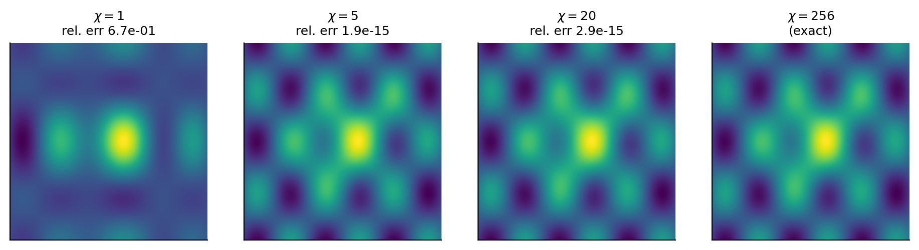
Figure 1.4: Rank-\(\chi\) truncations of a \(256\times256\) array, Eq. (1.123). A single outer product already captures the gross structure; twenty terms are visually indistinguishable from the original while storing eight per cent of the numbers.
The two panels of Figures 1.4 and 1.5 should be read together. The reconstructions show what is seen; the spectrum shows why. The singular values fall by three orders of magnitude within the first twenty indices, so the cumulative fraction of \(\|\bm{A}\|_F^2\) reaches \(0.999\) long before the rank is exhausted, and Eq. (1.124) guarantees that no other rank-\(\chi\) matrix does better. Whether a given data matrix admits such a truncation is a question about its singular value spectrum and about nothing else.
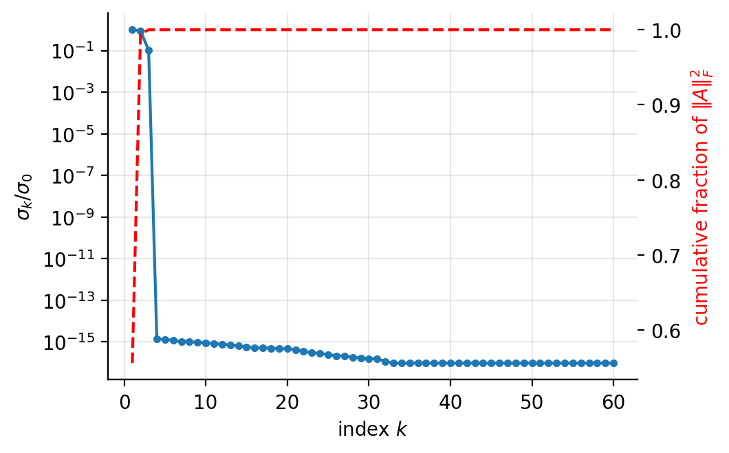
Figure 1.5: Singular value spectrum of the array of Figure 1.4 (left axis, logarithmic) and the cumulative fraction of \(\|\bm{A}\|_F^2\) retained by a rank-\(k\) truncation (right axis).
The theorem is the mathematical justification for a large part of applied machine learning. Compressing an image means truncating the SVD of its pixel matrix. Latent semantic analysis means truncating the SVD of a document-term matrix, so that documents and words are both represented in a \(\chi\)-dimensional space of “topics”. A recommender system means approximating a sparse user-item matrix \(\bm{R}\) by a product \(\bm{W}\bm{H}\) of low rank, the \(\chi\) retained directions being interpreted as latent tastes; the objective \(\|\bm{R}-\bm{W}\bm{H}\|_F^2\) is the Frobenius-norm minimisation of Section The Frobenius norm as a trace, and when all entries are observed its solution is exactly Eq. (1.123) truncated. And, as the next section shows, principal component analysis is the same construction applied to the centred design matrix.
import numpy as np

def truncated_svd(X, chi):
    """Best rank-chi approximation to X, with the retained variance."""
    U, s, Vt = np.linalg.svd(X, full_matrices=False)
    X_chi = (U[:, :chi] * s[:chi]) @ Vt[:chi]
    retained = np.sum(s[:chi]**2) / np.sum(s**2)
    return X_chi, retained

# Storage: n*p entries become chi*(n + p + 1)
n, p, chi = 512, 512, 40
print("compression ratio:", chi * (n + p + 1) / (n * p))
1.21. Principal component analysis#
Principal component analysis asks a question that sounds statistical and turns out to be algebraic: along which directions does the data vary most, and how many such directions are there?
Let \(\bm{X}_c\) be the centred design matrix of Section The covariance matrix. We look for the unit vector \(\bm{w}\) along which the projected data \(\bm{X}_c\bm{w}\) have the largest variance,
with \(\bm{\Sigma}\) the covariance matrix. Introducing a Lagrange multiplier for the constraint, the stationarity condition of \(\bm{w}^{T}\bm{\Sigma}\bm{w}-\lambda(\bm{w}^{T}\bm{w}-1)\) follows from Eq. (1.27) and reads
The maximising direction is therefore an eigenvector of the covariance matrix, and since \(\bm{w}^{T}\bm{\Sigma}\bm{w}=\lambda\) at any such point, the largest eigenvalue gives the largest variance. Repeating the argument in the subspace orthogonal to \(\bm{w}\) gives the second eigenvector, and so on. The principal directions are the eigenvectors of \(\bm{\Sigma}\) ordered by eigenvalue, and the eigenvalues are the variances along them. That is the entire content of PCA, and it is Eq. (1.54) read as a statement about data.
PCA through the SVD. In practice one never forms \(\bm{\Sigma}\). By Eq. (1.116) applied to \(\bm{X}_c=\bm{U}\bm{\Sigma}_{\!s}\bm{V}^{T}\) – writing \(\bm{\Sigma}_{\!s}\) for the matrix of singular values, to avoid a collision with the covariance matrix – the eigenvectors of \(\bm{\Sigma}=\bm{X}_c^{T}\bm{X}_c/(n-1)\) are the right singular vectors of \(\bm{X}_c\), and its eigenvalues are
The principal components – the coordinates of the observations in the new basis – are the columns of
and keeping only the first \(\chi\) of them is exactly the truncation of Section Low-rank approximation. Dimensionality reduction by PCA and best low-rank approximation are the same operation described in two vocabularies: Eq. (1.124) guarantees that no other \(\chi\)-dimensional linear projection retains more of the variance.
Going through the SVD rather than the covariance matrix is not a stylistic preference. By Eq. (1.118) forming \(\bm{X}_c^{T}\bm{X}_c\) squares the condition number, and the small eigenvalues – which are exactly the ones a scree plot is used to inspect – are the first casualties.
import numpy as np

def pca(X, n_components=None):
    """Principal component analysis through the SVD of the centred data.

    Returns the scores T, the principal directions V, and the explained
    variance ratio of each component.
    """
    Xc = X - np.mean(X, axis=0)                  # centre each feature
    U, s, Vt = np.linalg.svd(Xc, full_matrices=False)

    explained = s**2 / np.sum(s**2)
    k = n_components if n_components is not None else len(s)
    T = U[:, :k] * s[:k]                         # scores = Xc @ V
    return T, Vt[:k].T, explained[:k]
Two practical remarks. Centring is not optional: without it the first principal component points at the mean of the data and says nothing about their variability. Scaling, on the other hand, is a genuine choice. Because variance has units, a feature measured in millimetres will dominate one measured in metres purely through its numerical size; standardising every feature to unit variance before the decomposition performs PCA on the correlation matrix instead of the covariance matrix. Neither is universally right, but the choice must be made deliberately, and it must be made using training-set statistics only.
Machine learning connection
PCA is unsupervised: it never looks at \(\bm{y}\). The directions of largest variance in \(\bm{X}\) need not be the directions most useful for predicting the target, and it is entirely possible for the discriminating signal to lie along the last principal component. Principal component regression – fitting on the first \(\chi\) components – therefore works well when the informative directions happen to be the high-variance ones and badly when they do not. Partial least squares and linear discriminant analysis, which do consult the target, are the supervised answers to the same question, and we return to them in the chapter on dimensionality reduction.
1.22. Ridge regression through the singular value decomposition#
We close the chapter by returning to the regularised normal equations (1.42) with the SVD in hand, because the combination explains in two lines what Ridge regression does.
Substituting \(\bm{X}=\bm{U}\bm{\Sigma}\bm{V}^{T}\) into \((\bm{X}^{T}\bm{X}+\lambda\bm{I})\bm{\theta}=\bm{X}^{T}\bm{y}\) and using \(\bm{I}=\bm{V}\bm{V}^{T}\) gives \(\bm{V}(\tilde{\bm{\Sigma}}^2+\lambda\bm{I})\bm{V}^{T}\bm{\theta} = \bm{V}\bm{\Sigma}^{T}\bm{U}^{T}\bm{y}\), whence
Compare this with the ordinary least-squares result (1.122), in which the coefficient of \(\bm{u}_i^{T}\bm{y}\) was \(1/\sigma_i\). Ridge regression replaces
that is, it multiplies each term by a shrinkage factor \(\sigma_i^2/(\sigma_i^2+\lambda)\) lying between zero and one. Directions with \(\sigma_i^2\gg\lambda\) are left essentially untouched; directions with \(\sigma_i^2\ll\lambda\) are suppressed almost completely. The penalty acts selectively, and it acts hardest exactly where Eq. (1.122) was dividing by a dangerously small number.
The fitted values inherit the same structure. From \(\tilde{\bm{y}}=\bm{X}\bm{\theta}_{\mathrm{ridge}}\),
so the Ridge hat matrix is not a projector: its eigenvalues are the shrinkage factors rather than zeros and ones, and its trace,
decreases smoothly from \(p\) at \(\lambda=0\) towards zero as \(\lambda\to\infty\). This is the effective degrees of freedom promised in the notebox of Section Orthonormal bases and projections, and it makes precise the intuition that a regularised model is “smaller” than an unregularised one without having fewer parameters.
Truncated SVD regression, by contrast, replaces \(1/\sigma_i\) by zero below a cutoff and leaves it alone above: a hard threshold where Ridge applies a soft one. The two are the same idea applied with different degrees of politeness, and both are, in the end, statements about the singular values of the design matrix. We take up the statistical consequences – the bias each introduces, the variance each removes, and how to choose \(\lambda\) – in Chapter 3.
1.23. Summary and the programs#
The chapter has moved from notation to algorithms. The algebra of Sections Notation and conventions-The covariance matrix supplies the language in which machine learning is written: a data set is a design matrix, a linear model is a matrix acting on a parameter vector, fitting is projection onto a column space, differentiating a cost function is matrix calculus, and the structure of a data set is the spectrum of its covariance matrix. The numerical sections supply the means of extracting numbers from that language.
Three dividing lines are worth keeping in mind. The first separates direct from iterative methods. Direct methods – Gaussian elimination, LU, Cholesky, the Householder-based eigenvalue and SVD routines – deliver the complete answer in a fixed \(\bigO(n^3)\) number of operations and require the matrix to be stored. Iterative methods – Jacobi, Gauss-Seidel, over-relaxation, conjugate gradient, the Krylov eigensolvers – deliver an approximation that improves with each step and require only the action of the matrix on a vector. Every large-scale method in this book, gradient descent included, lives on the second side of that line.
The second line separates well-conditioned from ill-conditioned problems. The condition number \(\kappa_2(\bm{X})=\sigma_0/\sigma_{r-1}\) is a property of the data, not of the algorithm, and it decides how much of the input precision survives. Since \(\kappa_2(\bm{X}^{T}\bm{X})=\kappa_2(\bm{X})^2\), an algorithm that forms the normal equations pays twice; this is why the least-squares routines one should actually call are built on the QR decomposition or the SVD.
The third line is the one drawn by the singular value decomposition, and it is of a different kind. It separates the part of a problem that carries information from the part that does not. The same list of singular values tells us the numerical rank of a design matrix, how far a set of features is from collinearity, how much of the variance a \(\chi\)-dimensional projection retains, how well a recommender matrix can be factorised, and how strongly Ridge regression will shrink each direction. Sections The singular value decomposition-Ridge regression through the singular value decomposition are five readings of one decomposition, and the thread connecting them – Eq. (1.124), that truncating the singular values is the best approximation of its rank – runs through the rest of this book.
The complete programs are collected in doc/BookML/BookPrograms:
direct_solvers.py– Gaussian elimination, LU and Cholesky, with determinants and inverses.iterative_solvers.py– Jacobi, Gauss-Seidel, over-relaxation and the conjugate gradient method, in both a matrix-based and a matrix-free form.eigenvalues.py– the power method, inverse iteration and the Rayleigh quotient, together with the timing comparisons against the LAPACK routines quoted in Section What library routines actually do.svd_tools.py– the singular value decomposition applied to rank determination, the pseudoinverse, truncated least squares, low-rank approximation, principal component analysis and Ridge regression, including the collinear design matrix of Section Rank, the pseudoinverse and ill-conditioned design matrices and the accuracy comparison of Table 1.2.
Each file runs as a script and reproduces the numbers quoted in this chapter. An executable version of the same material, in which the reader can vary the parameters, is available as a Jupyter notebook in the accompanying Jupyter-book.
1.24. Exercises#
1.24.1. Warm-up exercises#
Inner and outer products. Let \(\bm{u}=\begin{bmatrix}1 & 2 & -1\end{bmatrix}^{T}\) and \(\bm{v}=\begin{bmatrix}3 & 0 & 1\end{bmatrix}^{T}\). (a) Compute \(\bm{u}^{T}\bm{v}\) and \(\|\bm{u}\|_1\), \(\|\bm{u}\|_2\), \(\|\bm{u}\|_{\infty}\). (b) Compute the outer product \(\bm{u}\bm{v}^{T}\) and verify that \(\mathrm{Tr}(\bm{u}\bm{v}^{T})=\bm{v}^{T}\bm{u}\). (c) What is the rank of \(\bm{u}\bm{v}^{T}\)? Justify your answer without computing a determinant.
Special matrix types. For each matrix below, identify which type(s) from Table 1.1 it belongs to, and verify your answer using the element conditions in the table: (a) a rotation by an angle \(\theta\) in the plane, \(\bm{R}=\begin{bmatrix}\cos\theta&-\sin\theta\\ \sin\theta&\cos\theta\end{bmatrix}\); (b) any covariance matrix; (c) \(\bm{H}=\frac{1}{\sqrt{2}} \begin{bmatrix}1&1\\1&-1\end{bmatrix}\).
Projectors. Let \(\bm{q}\in\mathbb{R}^{n}\) with \(\|\bm{q}\|_2=1\) and set \(\bm{P}=\bm{q}\bm{q}^{T}\). (a) Verify \(\bm{P}^{T}=\bm{P}\) and \(\bm{P}^{2}=\bm{P}\). (b) Show that the eigenvalues of \(\bm{P}\) are \(1\) (once) and \(0\) (\(n-1\) times), and that \(\mathrm{Tr}(\bm{P})=1\). (c) Show that \(\bm{I}-\bm{P}\) is also a projector and that \(\bm{P}(\bm{I}-\bm{P})=\bm{0}\).
Matrix calculus. Using only Eqs. (1.25) and (1.27), compute (a) \(\partial\left(\bm{a}^{T}\bm{x}\bm{b}^{T}\bm{x}\right)/\partial\bm{x}\); (b) \(\partial\|\bm{x}-\bm{a}\|_2^{2}/\partial\bm{x}\); (c) the gradient and the Hessian of \(C(\bm{\theta})=\|\bm{y}-\bm{X}\bm{\theta}\|_2^{2} +\lambda\|\bm{\theta}\|_2^{2}\), and use them to confirm Eq. (1.42).
Positive semi-definiteness. (a) Show that \(\bm{X}^{T}\bm{X}\) is positive semi-definite for any \(\bm{X}\). (b) Show that it is positive definite if and only if the columns of \(\bm{X}\) are linearly independent. (c) Deduce that if \(p>n\) the least-squares problem cannot have a unique solution, and explain what Eq. (1.122) returns instead.
Trace identities. (a) Prove \(\mathrm{Tr}(\bm{A}\bm{B})=\mathrm{Tr}(\bm{B}\bm{A})\) directly from the definition, and note that \(\bm{A}\bm{B}\) and \(\bm{B}\bm{A}\) need not even have the same dimensions. (b) Use it to prove \(\|\bm{A}\|_F^2=\mathrm{Tr}(\bm{A}^{T}\bm{A}) =\mathrm{Tr}(\bm{A}\bm{A}^{T})\). (c) Show that \(\|\bm{Q}\bm{A}\|_F=\|\bm{A}\|_F\) for orthogonal \(\bm{Q}\).
Conditioning in practice (numerical). Build a design matrix whose columns are \(1,x,x^2,\dots,x^{d-1}\) for \(100\) points \(x\) equally spaced on \([0,1]\) – the Vandermonde matrix of a polynomial fit. (a) Compute \(\kappa_2(\bm{X})\) for \(d=2,4,\dots,14\) and plot it on a logarithmic scale. (b) For which \(d\) does \(\kappa_2(\bm{X}^{T}\bm{X})\) exceed \(1/\varepsilon\)? (c) Repeat with the columns rescaled to unit norm, and comment.
Least squares three ways (numerical). For the collinear design matrix of Section Rank, the pseudoinverse and ill-conditioned design matrices, compute \(\bm{\theta}\) in three ways: (a) by solving the normal equations with
np.linalg.solve; (b) withnp.linalg.lstsq; and (c) with the truncated SVD of the same section. Compare the coefficients, the training error and the predictions. Which two agree, and why?Spectral decomposition. Let \(\bm{A}=\begin{bmatrix}2&1\\1&2\end{bmatrix}\). (a) Find its eigenvalues and normalised eigenvectors. (b) Write the spectral decomposition \(\bm{A}=\sum_i\lambda_i\bm{v}_i\bm{v}_i^{T}\) explicitly and verify it by multiplying out. (c) Compute \(\bm{A}^{1/2}\) and \(\bm{A}^{-1}\) using Eq. (1.56), and check the latter against a direct inversion.
PCA by hand (numerical). Generate \(n=500\) points in \(\mathbb{R}^{2}\) from a Gaussian with covariance \(\begin{bmatrix}3&2\\2&2\end{bmatrix}\). (a) Compute the covariance matrix of the sample and its eigendecomposition. (b) Compute the SVD of the centred data and verify Eq. (1.127). (c) Plot the data with the two principal directions drawn as arrows scaled by \(\sqrt{\lambda_i}\). (d) Repeat after multiplying the first coordinate by \(100\). What happens to the principal directions, and what does this tell you about scaling?
1.24.2. Exercise session, week 34: orthogonal transformations, least squares and the SVD#
The exercises of this session are meant as reminders of the specific linear algebra elements that we shall use throughout the course, and as a first encounter with the least-squares problem that occupies Chapter 3.
Exercise 1: orthogonal transformations and invariance. It is common in data analysis to express the data in a new basis. Principal component analysis, the discrete Fourier transform and the whitening transformation of Eq. (1.59) are all of this kind, and in each case the change of basis is described by an orthogonal (or, for complex data, unitary) matrix.
Assume that \(\bm{Q}\) is orthogonal with dimension \(n\times n\) and matrix elements \(q_{ij}\), and that \(\{\bm{\phi}_{\lambda}\}\) is an orthonormal basis of \(\mathbb{R}^{n}\) which diagonalises a symmetric matrix \(\bm{O}\),
Define a new set of vectors by \(\bm{\psi}_p=\bm{Q}\bm{\phi}_p\).
Exercise 2: the normal equations. Consider the linear model \(\tilde{\bm{y}}=\bm{X}\bm{\theta}\) with \(\bm{X}\in\mathbb{R}^{n\times p}\) and the cost function \(C(\bm{\theta})=\|\bm{y}-\bm{X}\bm{\theta}\|_2^{2}\).
Exercise 3: the SVD and rank. Let \(\bm{X}=\bm{U}\bm{\Sigma}\bm{V}^{T}\) be the singular value decomposition of an \(n\times p\) matrix.