
13. Chapter 13: Transformers#
Each architecture in this book has been a restriction of the dense layer, justified by a property of the data. Chapter 10 imposed locality and translation equivariance and obtained convolution; Chapter 11 imposed sequential processing with a carried state and obtained recurrence. In each case a fixed interaction pattern was written into the architecture before any data were seen: a convolutional layer couples a pixel to its neighbours whatever the image contains, and a recurrent layer couples each step to the previous one whatever the sequence says.
The transformer takes the opposite decision. It couples every element to every other element, and it lets the strength of each coupling be computed from the data at run time. The interaction pattern is not designed; it is inferred, afresh for every input. That single change of principle – from fixed couplings to adaptive couplings – is what this chapter is about, and it turns out to have consequences that are mathematically sharp, physically suggestive, and occasionally limiting in ways worth knowing.
This chapter follows the transformer lecture notes for the course. We derive attention, prove the properties that characterise it, implement it from scratch with verified gradients, and measure two things that matter: why the \(1/\sqrt{d_k}\) in Eq. (13.5) is not cosmetic, and what a single attention layer provably cannot compute.
13.1. Tokens#
A transformer consumes a sequence of vectors,
called tokens, and returns another sequence of the same length, \((\bm{y}_1,\dots,\bm{y}_n)\). What a token is depends on the problem: a word in a sentence, a patch of an image, a node of a discretised field, or a sample of a solution to a partial differential equation. Collect them as the rows of \(\bm{X}\in\mathbb{R}^{n\times d}\).
The generality is the point. Anything that can be cut into pieces and given a vector description can be handed to a transformer, and the architecture makes no assumption about how the pieces are arranged. As Theorem 13.2 will prove, it makes no assumption about their order either, which is a liberation and a problem in equal measure.
13.2. Scaled dot-product attention#
For each position \(i\) we want an output that is a weighted combination of information drawn from all positions,
with weights \(A_{ij}\) that depend on the data. Three learned linear maps supply the ingredients. From each token we form a query, a key and a value,
with \(\bm{W}_Q,\bm{W}_K\in\mathbb{R}^{d\times d_k}\) and \(\bm{W}_V\in\mathbb{R}^{d\times d_v}\). The reading is worth memorising: the query is what position \(i\) is looking for, the key is what position \(j\) advertises, and the value is what position \(j\) contributes if selected.
The weight is the softmax of the query-key inner product,
In matrix form, with \(\bm{Q}=\bm{X}\bm{W}_Q\), \(\bm{K}=\bm{X}\bm{W}_K\) and \(\bm{V}=\bm{X}\bm{W}_V\),
The \(n\times n\) matrix \(\bm{Q}\bm{K}^{\mathsf{T}}\) holds the interaction between every pair of positions; the softmax normalises each row; multiplication by \(\bm{V}\) aggregates. When \(\bm{Q}\), \(\bm{K}\) and \(\bm{V}\) all come from the same \(\bm{X}\), as here, this is self-attention.
13.2.1. What attention is#
Three statements characterise Eq. (13.5), and each has a consequence that is easy to state and easy to forget.
Proposition 13.1 (Attention averages)
The matrix \(\bm{A}\) of Eq. (13.4) is row-stochastic: \(A_{ij}>0\) and \(\sum_j A_{ij}=1\) for every \(i\). Consequently each output \(\bm{y}_i\) lies in the convex hull of the value vectors \(\{\bm{v}_1,\dots,\bm{v}_n\}\).
Proof
Positivity is immediate from the exponential, and the denominator of Eq. (13.4) is exactly the sum of the numerators over \(j\), so the rows sum to one. A combination with non-negative coefficients summing to one is by definition a convex combination, and Eq. (13.2) exhibits \(\bm{y}_i\) as one.
The consequence is a genuine limitation. A single attention layer cannot produce an output outside the convex hull of its own values: it can select, blend and interpolate, but it cannot extrapolate. This is one reason the feed-forward sublayer of Section Multi-head attention and the transformer block is not an optional extra – without it a stack of attention layers would be confined to convex hulls forever.
Theorem 13.2 (Permutation equivariance)
Let \(\bm{\Pi}\) be an \(n\times n\) permutation matrix. Then self-attention satisfies
The output at a position depends on the set of tokens and on which token sits at that position, but not on the order of the others.
Proof
The three maps of Eq. (13.3) act on each row independently, so \(\bm{\Pi}\bm{X}\) produces \(\bm{\Pi}\bm{Q}\), \(\bm{\Pi}\bm{K}\) and \(\bm{\Pi}\bm{V}\). The score matrix becomes \((\bm{\Pi}\bm{Q})(\bm{\Pi}\bm{K})^{\mathsf{T}}/\sqrt{d_k} =\bm{\Pi}\bm{S}\bm{\Pi}^{\mathsf{T}}\). A row-wise softmax commutes with a permutation of the rows, and permuting the columns of a row permutes the entries of that row’s softmax identically, so \(\mathrm{softmax}(\bm{\Pi}\bm{S}\bm{\Pi}^{\mathsf{T}}) =\bm{\Pi}\,\mathrm{softmax}(\bm{S})\,\bm{\Pi}^{\mathsf{T}}\). Finally \(\bm{\Pi}\bm{A}\bm{\Pi}^{\mathsf{T}}\bm{\Pi}\bm{V}=\bm{\Pi}\bm{A}\bm{V}\), using \(\bm{\Pi}^{\mathsf{T}}\bm{\Pi}=\bm{I}\).
Compare Theorem 10.7, which said convolution is the unique linear map equivariant to translation. Attention is equivariant to the much larger group of all permutations, and a larger symmetry group means a weaker model: attention knows nothing about order at all. For a sentence or a time series that is unacceptable, and Section Masking and position puts the order back in by hand.
Proposition 13.3 (Cost)
Computing Eq. (13.5) requires \(\bigO(n^{2}d_k+n^{2}d_v)\) arithmetic operations and \(\bigO(n^{2})\) memory for the matrix \(\bm{A}\).
Proof
\(\bm{Q}\bm{K}^{\mathsf{T}}\) is a product of an \(n\times d_k\) and a \(d_k\times n\) matrix, costing \(\bigO(n^{2}d_k)\); the softmax is \(\bigO(n^{2})\); and \(\bm{A}\bm{V}\) costs \(\bigO(n^{2}d_v)\).
The quadratic scaling in sequence length is the central practical difficulty of the architecture, and the reason for a large literature on sparse, low-rank and kernelised approximations. Contrast a convolution, which by Eq. (10.18) touches only \(F^{2}\) neighbours per position, and a recurrent layer, which is linear in \(n\) but strictly sequential and therefore cannot be parallelised across time. Attention buys global access and parallelism, and pays for both in \(n^{2}\).
\subsection{Why the \texorpdfstring{\(1/\sqrt{d_k}\)}{1/sqrt(dk)}}
The scaling in Eq. (13.5) looks like a detail. It is not, and the reason can be made precise.
Proposition 13.4 (Variance of the logits)
Let \(\bm{q},\bm{k}\in\mathbb{R}^{d_k}\) have independent entries with mean zero and variance \(\sigma^{2}\). Then
so the logits have standard deviation \(\sigma^{2}\sqrt{d_k}\), growing without bound with the head dimension. Dividing by \(\sqrt{d_k}\) makes the variance independent of \(d_k\).
Proof
\(\bm{q}\cdot\bm{k}=\sum_{r}q_rk_r\) is a sum of \(d_k\) independent terms, each of mean \(\mathbb{E}[q_r]\mathbb{E}[k_r]=0\) and variance \(\mathbb{E}[q_r^{2}k_r^{2}]-0=\sigma^{4}\) by independence. Variances of independent variables add.
Measured with \(\sigma^{2}=1\) over \(4000\) samples:
  d_k    Var(q.k) unscaled   Var(q.k) scaled   prediction d_k
      4              4.22            1.0538             4
     16             15.87            0.9916            16
     64             61.48            0.9607            64
    256            251.83            0.9837           256
   1024           1011.47            0.9878          1024
The middle column tracks the last one over three decades, and the scaled variant sits at one throughout. Figure 13.1(a) plots it.
That is the statistics. The reason it matters is what large logits do to the softmax. As the spread of the scores grows, the softmax approaches a hard maximum: one weight goes to one, the rest to zero, and the derivative goes to zero with them. Measuring the Frobenius norm of the softmax Jacobian for logits drawn from \(\mathcal{N}(0,c^{2})\):
  scale   max A     entropy    ||d softmax/d s||_F
   0.25  0.06851    3.4214   4.808e-02
   1.00  0.37786    2.4937   1.029e-01
   4.00  0.98926    0.0703   8.223e-03
  16.00  1.00000    0.0000   1.745e-09
  64.00  1.00000    0.0000   3.276e-36
Between \(c=1\) and \(c=64\) the gradient falls by thirty-five orders of magnitude. A network whose attention weights sit in that regime receives no gradient through them at all and cannot learn what to attend to. Since Proposition 13.4 says \(c\) grows as \(\sqrt{d_k}\), a model with \(d_k=64\) and unscaled logits starts life at \(c\approx8\), already well into the saturated region. The \(1/\sqrt{d_k}\) is what keeps it at \(c\approx1\).
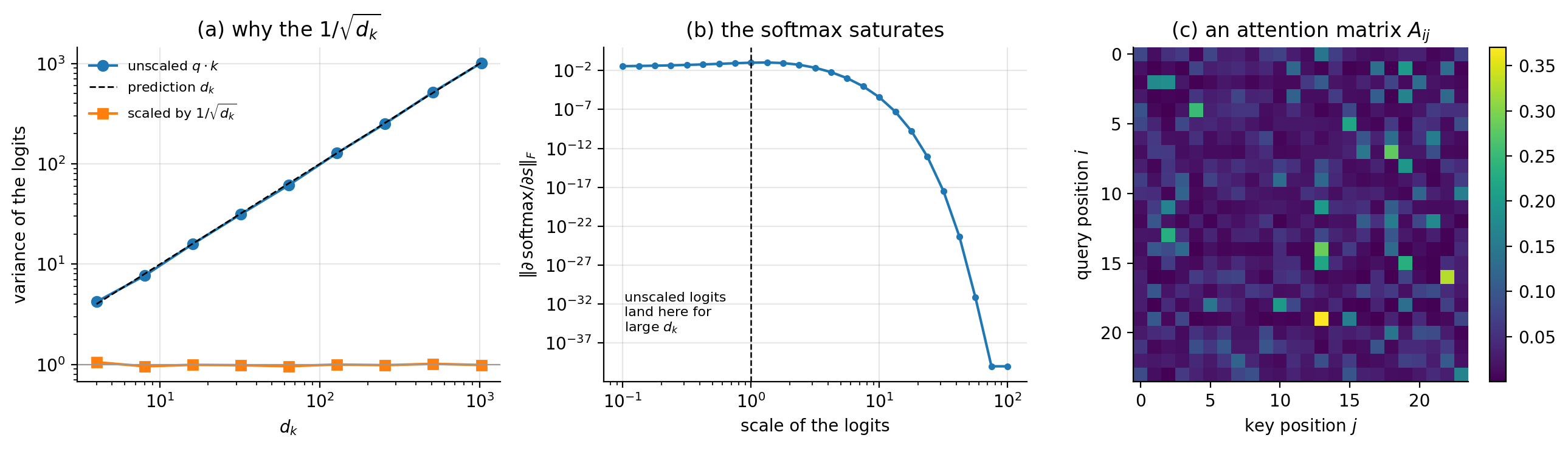
Figure 13.1: (a) Variance of the attention logits against head dimension. The unscaled dot product follows the prediction \(d_k\) of Proposition 13.4 exactly; dividing by \(\sqrt{d_k}\) flattens it to one. (b) Frobenius norm of the softmax Jacobian against the scale of the logits: past a scale of about four the softmax saturates and the gradient collapses, reaching \(10^{-36}\) by scale \(64\). (c) An attention matrix \(A_{ij}\) for an untrained network: every row sums to one, by Proposition 13.1.
The same failure as Chapter 11, at a different place
Section Why long sequences are hard showed gradients vanishing through a product of Jacobians along a sequence. Here they vanish through a single saturated softmax. Both are cured by keeping a quantity at scale one – the spectral radius there, the logit variance here – and in both cases the cure is a choice of scaling made before training rather than an adjustment made during it. This is the recurring lesson of Chapters 8 to 13: deep networks are trained by controlling scales.
13.3. Masking and position#
Masks. Sometimes a position must not see another. In autoregressive generation, the prediction at step \(i\) may depend only on steps \(j\le i\), or the model would be allowed to read its own answer. This is imposed by adding a mask to the scores before the softmax,
so that \(\exp(s_{ij})=0\) above the diagonal and \(\bm{A}\) becomes lower triangular. The implementation adds \(-\infty\) rather than deleting entries so that the shape of the computation is unchanged.
A mask destroys Theorem 13.2, and deliberately: the whole purpose is to make position \(i\) different from position \(j\). We verify both facts in Section Implementation and verification.
Positional encodings.
Theorem 13.2 says a transformer without further information cannot distinguish a sentence from an anagram of it. The standard remedy is to add a position-dependent vector to each token before the first block. The sinusoidal choice of the original architecture is
for position \(m\) and channel \(r\), and \(\bm{x}_m \leftarrow \bm{x}_m +\mathrm{PE}(m,\cdot)\). The construction is a bank of sinusoids at geometrically spaced frequencies, so that low channels vary slowly across the sequence and high channels vary fast – a positional analogue of the multiscale argument of Section Pooling.
Its useful property is usually stated loosely – that the inner product \(\mathrm{PE}(m)\cdot\mathrm{PE}(m')\) depends mainly on \(m-m'\). It is in fact exact, and the exactness is the whole reason for choosing sinusoids rather than any other bank of position-dependent features.
Proposition 13.5 (The sinusoidal encoding is a relative code)
Write \(\omega_r=10000^{-2r/d}\) for \(r=0,\dots,d/2-1\). For the encoding Eq. (13.9),
(shift is a fixed rotation) for every offset \(k\) there is an orthogonal matrix \(\bm{R}_k\), independent of \(m\), with
\[ \mathrm{PE}(m+k) = \bm{R}_k\,\mathrm{PE}(m) \qquad\text{for all } m,\tag{13.10} \]namely the block-diagonal matrix whose \(r\)th block is the plane rotation through \(\omega_r k\);
(the kernel is exactly relative)
\[ \mathrm{PE}(m)\cdot\mathrm{PE}(m') = \sum_{r=0}^{d/2-1}\cos\!\left(\omega_r\left(m-m'\right)\right),\tag{13.11} \]a function of \(m-m'\) alone, with maximum \(d/2\) at \(m=m'\).
Proof
For channel pair \(r\) the encoding is \((\sin\omega_r m,\cos\omega_r m)\), a point on the unit circle at angle \(\omega_r m\) measured from the vertical. The angle-addition formulae give
whose matrix depends on \(k\) and not on \(m\); stacking the blocks gives Eq. (13.10), and each block is a rotation so \(\bm{R}_k\) is orthogonal. For (ii), the \(r\)th pair contributes \(\sin\omega_r m\sin\omega_r m'+\cos\omega_r m\cos\omega_r m' =\cos(\omega_r(m-m'))\), and summing over \(r\) gives Eq. (13.11); each cosine is at most one, attained together only at \(m=m'\).
Both parts matter. Equation (13.11) says the encoding supplies the dot product of Eq. (13.4) with an exact function of relative distance, so a relative notion of position is available without ever being written down – Figure 13.2(c) is a plot of it. Equation (13.10) says something stronger and less often noted: because translation acts linearly on the encoding, a query matrix \(\bm{W}_Q\) can implement “attend to whatever is \(k\) places back” as a single linear map, valid at every position at once. That is what makes the previous-token head of Section What one attention layer cannot do easy to learn, and it is exactly the property a learned positional embedding does not have. Learned embeddings and explicit relative encodings are the two common alternatives, and the first of them pays for its freedom in Section PyTorch and TensorFlow.
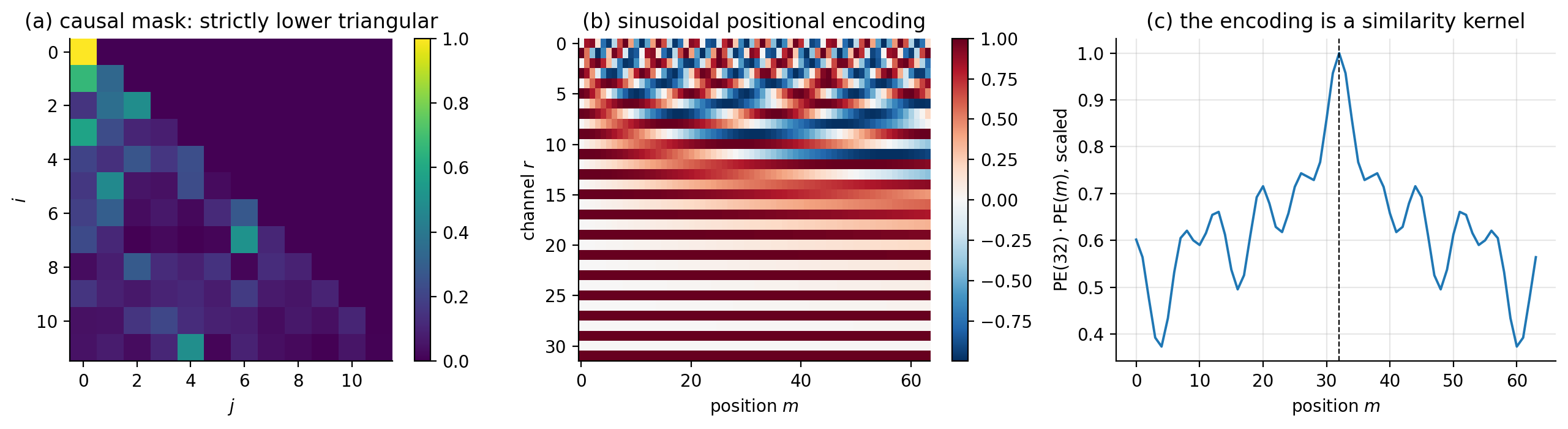
Figure 13.2: (a) An attention matrix under the causal mask of Eq. (13.8): the strict upper triangle is exactly zero, measured to \(0\). (b) The sinusoidal positional encoding of Eq. (13.9), channels against position; low channels vary slowly, high channels fast. (c) The inner product of the encoding at position \(32\) with every other position: a similarity kernel peaked on the diagonal, which is how relative distance reaches the dot product of Eq. (13.4).
13.4. Multi-head attention and the transformer block#
One attention matrix imposes a single pattern of couplings. Real problems have several – syntactic and semantic in language, local and long-range in a field. Multi-head attention runs \(H\) attentions in parallel with separate projections and mixes the results:
Taking \(d_k=d_v=d/H\) keeps the cost of \(H\) heads equal to that of one head of full width, so multiple heads are free. Different heads reliably learn different patterns, and inspecting them is the beginning of interpretability work.
The block. Attention is one sublayer of a transformer block, which also contains a position-wise feed-forward network, residual connections and normalisation. In the pre-norm arrangement now standard,
where the MLP is applied to each token separately, \(\mathrm{MLP}(\bm{z})=\bm{W}_2\,\mathrm{GELU}(\bm{W}_1\bm{z}+\bm{b}_1)+\bm{b}_2\), with the GELU activation of Section Activation functions, and layer normalisation acts across the feature axis of each token,
Each ingredient earns its place. The MLP supplies the non-linearity that Proposition 13.1 showed attention alone lacks, and it is where most of the parameters live. The residual connections give the gradient an undamped path from the loss to every layer – precisely the additive path that Eq. (11.29) gave the LSTM cell state. Layer normalisation keeps the scale of the activations fixed, which by Section Why the \texorpdfstring{\(1/\sqrt{d_k}\)}{1/sqrt(dk)} is what the softmax needs.
A transformer is a stack of these blocks. Nothing in it is unfamiliar: it is attention, plus the multilayer perceptron of Chapter 8, plus residual connections and normalisation.
13.5. Implementation and verification#
We write attention with autograd rather than by hand, for the reason Section Automatic differentiation gave: differentiating a softmax nested inside two matrix products is exactly the error-prone drudgery automatic differentiation exists to remove.
def softmax_rows(S):
    """Row-wise softmax, shifted for stability."""
    S = S - np.max(S, axis=-1, keepdims=True)
    E = np.exp(S)
    return E / np.sum(E, axis=-1, keepdims=True)


def attention(Q, K, V, mask=None):
    """Scaled dot-product attention, Eq. (13.attention).

    Q is (n, d_k), K is (m, d_k), V is (m, d_v); the output is (n, d_v).
    """
    d_k = Q.shape[-1]
    S = Q @ K.T / np.sqrt(d_k)                 # (n, m) scores
    if mask is not None:
        S = S + mask                           # -inf where attention is banned
    A = softmax_rows(S)                        # (n, m), rows sum to one
    return A @ V, A
Multi-head attention loops over heads, concatenates and mixes; the block adds the residuals and normalisation of Eq. (13.14).
def block(P, X, mask=None):
    """Pre-norm transformer block, Eq. (13.block).

    X -> X + MHA(LN(X)) -> X + MLP(LN(X)).  The residual paths carry the
    identity, which is what keeps deep stacks trainable (cf. Section 11.lstmwhy).
    """
    Y, A = multihead(P, layernorm(X, P["g1"], P["be1"]), mask)
    X = X + Y
    Z = layernorm(X, P["g2"], P["be2"])
    X = X + gelu(Z @ P["W1"] + P["b1"]) @ P["W2"] + P["b2"]
    return X, A
The checks follow the propositions one by one.
rows of A sum to 1 : 2.22e-16
A >= 0             : True
head output within the bounding box of V : True

=== permutation equivariance:  Att(PX) = P Att(X) ===
  trial 0: max|Att(PX) - P Att(X)| = 1.67e-16
  trial 1: max|Att(PX) - P Att(X)| = 3.33e-16
  trial 2: max|Att(PX) - P Att(X)| = 2.22e-16

=== a causal mask breaks it (as it must) ===
  max|Att(PX) - P Att(X)| with mask = 1.897e+00
  attention matrix upper triangle (should be 0): 0.00e+00
Proposition 13.1 and Theorem 13.2 hold to machine precision, and the mask does exactly what Eq. (13.8) says: it zeroes the upper triangle exactly and destroys the equivariance completely. The batched implementation used for training agrees with the looped one to \(8.9\times10^{-16}\).
13.6. What one attention layer cannot do#
Theorem 13.2 and Proposition 13.1 are statements about what attention is. This section is about what a given depth of it can compute, and the answer is sharper than one might guess.
Consider associative recall. A sequence presents \(L\) key-value pairs \(k_1v_1k_2v_2\cdots k_Lv_L\) and then repeats one of the keys; the model must emit the value that followed it. The task is trivial for a human, has an exact algorithm, and requires reaching a specific earlier position whose distance grows with \(L\). It is the cleanest test of global access there is.
Now look at what one attention layer can do with it. The query at the final position carries the repeated key, and the dot product of Eq. (13.4) can certainly make it match the earlier position holding the same key. But matching that position retrieves that position’s value vector – the key – and what is wanted is the token one place to the right. A single layer has no way to attend to one position and read from another.
It needs two. The first layer copies each token’s predecessor into its representation; the second matches the query against keys and now finds the value already attached. This composition is known as an induction head, and it is a mechanism rather than a metaphor. The informal argument above can be made into a statement with a proof.
Proposition 13.6 (One content-matching layer cannot do associative recall)
Consider a single attention layer in which the key and value at position \(j\) depend only on the symbol \(s_j\) there, \(\bm{k}_j=K(s_j)\) and \(\bm{v}_j=V(s_j)\), the query at the final position depends only on \(s_T\), and position enters the scores only through an additive bias \(b_{Tj}\) that does not depend on the symbols. Let the recall task be as above, with the \(L\) keys distinct, the \(L\) values drawn independently and uniformly, and the query \(s_T=s_{2q-1}\) for a uniformly chosen \(q\). Then the layer cannot solve the task better than chance in the limit of large vocabulary.
Proof
The attention weight on position \(j\) is \(\alpha_j\propto\exp\bigl(Q(s_T)\cdot K(s_j)+b_{Tj}\bigr)\), so it is a function of the pair \((s_T,s_j)\) and of \(j\). The answer required is \(V(s_{2q})\), the value following the matched key, so the layer must place its mass on position \(2q\). But \(s_{2q}\) is drawn independently of \(s_{2q-1}=s_T\) and of every other symbol, so \(Q(s_T)\cdot K(s_{2q})\) carries no information about whether \(2q\) is the position wanted; and \(b_{T,2q}\) is the same for all instances with the same \(q\), which is unknown to the layer. Hence \(\mathbb{E}[\alpha_{2q}]\) is the same for every value position, the output is an average of \(V\) over value symbols independent of the query, and the readout can do no better than the marginal. A vocabulary of size \(M\) makes that \(1/M\).
Two layers escape the proposition by breaking its hypothesis. A first layer whose attention pattern is positional rather than content-based – attend one place back, which by Eq. (13.10) is a single linear map on the encoding – writes \(s_{j-1}\) into position \(j\). After that the key at position \(2q\) is a function of \(s_{2q-1}=s_T\), the hypothesis \(\bm{k}_j=K(s_j)\) no longer holds, and content matching at the second layer finds exactly the position wanted.
So the prediction is sharp: one block fails and two succeed. We test it, with a vocabulary of eight symbols, so that chance is \(0.125\).
\noalign{} \(L\) |
Model |
Parameters |
Test accuracy |
|---|---|---|---|
\noalign{}\noalign{} \(2\) |
transformer, 1 block |
\(8928\) |
\(1.000\) |
\(2\) |
RNN (Chapter 11) |
\(8858\) |
\(1.000\) |
\noalign{}\noalign{} \(4\) |
transformer, 1 block |
\(8928\) |
\(0.366\) (\(0.352\)–\(0.380\)) |
\(4\) |
RNN (Chapter 11) |
\(8858\) |
\(0.351\) (\(0.333\)–\(0.370\)) |
\(4\) |
transformer, 2 blocks |
\(17344\) |
\(\mathbf{0.993}\) (\(0.985\)–\(1.000\)) |
\noalign{} |
Table 13.1: Associative recall with \(L\) key-value pairs, so sequence length \(T=2L+1\). All models trained by Adam with \(\gamma=3\times10^{-3}\) on freshly generated batches; accuracy on \(400\) unseen sequences, ranges over two seeds. Chance is \(0.125\).
At \(L=2\) the sequence is five tokens long and everything works. At \(L=4\) both the one-block transformer and the recurrent network of Chapter 11 sit at about \(0.36\), well above chance but nowhere near the task, and they sit there for three thousand updates. Adding a second block takes the same architecture to \(0.993\).
This is worth dwelling on, because it cuts against the usual way of describing transformers. Global access is not sufficient. The one-block model can already see every position – Proposition 13.3 charges it \(n^{2}\) for the privilege – and it still cannot solve a task that a two-line program solves, because the computation it needs is a composition of two retrievals and it has only one layer in which to do them. Depth is not a way of adding capacity here; it is a way of adding steps.
An honest reading of the middle rows
The one-block transformer does not beat the recurrent network on this task; the two are statistically indistinguishable at \(0.366\) against \(0.351\). A comparison stopped there would conclude that attention offers nothing. The right conclusion is that the architecture was mismatched to the computation, and the fix was depth rather than width or attention span. When a model plateaus well above chance, it is worth asking what algorithm it would need and how many sequential steps that algorithm takes.
13.7. Comparisons and interpretations#
13.7.1. Against the other architectures#
The four architectures of Chapters 8 to 13 differ in exactly one respect: which elements interact, and how strongly.
\noalign{} Architecture |
Coupling \(y_i=\sum_j C_{ij}x_j\) |
Cost per layer |
|---|---|---|
\noalign{}\noalign{} MLP |
\(C_{ij}=W_{ij}\), dense and fixed |
\(\bigO(n^{2}d^{2})\) |
CNN |
\(C_{ij}=w_{i-j}\), local and fixed |
\(\bigO(nF d^{2})\) |
RNN |
\(C\) lower triangular, applied step by step |
\(\bigO(nd^{2})\), sequential |
Transformer |
\(C_{ij}=A_{ij}(\bm{X})\), dense and adaptive |
\(\bigO(n^{2}d)\) |
\noalign{} |
An MLP has fixed weights \(\bm{W}\) that do not depend on the input. A convolution is the special case in which those weights are local and shared, by Theorem 10.2. A recurrent layer reaches distant positions only by composing many short steps, which is what Theorem 11.1 punishes. Attention alone lets the coupling matrix be a function of the data:
That is the whole of the innovation, and everything else in the architecture is scaffolding to make it trainable.
13.7.2. A statistical-mechanics reading#
Equation (13.4) will look familiar to anyone who has met a canonical ensemble. Writing \(E_{ij}=-s_{ij}\),
which is a Gibbs distribution over interaction partners at inverse temperature one, with \(Z_i\) a per-query partition function. The scores are effective energies; the softmax is a local Boltzmann weighting; and the \(1/\sqrt{d_k}\) of Section Why the \texorpdfstring{\(1/\sqrt{d_k}\)}{1/sqrt(dk)} is a choice of temperature, with saturation being the zero-temperature limit in which the distribution collapses onto its ground state.
The aggregation step then reads
which is a mean-field update with state-dependent couplings. In an Ising or Hopfield model the \(J_{ij}\) are fixed by the Hamiltonian; here they are recomputed from the current configuration at every layer. A transformer is, in this reading, a nonlinear adaptive mean-field model, and the analogy is close enough to have been productive: the connection between attention and modern Hopfield networks with exponential capacity is more than superficial.
13.7.3. Kernels and graphs#
Equation (13.2) also reads as a discretised integral operator,
with the difference that \(K\) is learned rather than prescribed. Compare the kernel methods of Chapter 6, where \(K\) was chosen in advance and the representer theorem then fixed everything: attention learns the kernel and gives up the theory.
Viewed as a graph, attention defines a complete weighted graph on the tokens with edge weights \(A_{ij}\), which makes a transformer a graph neural network whose graph is inferred rather than given. A message-passing network on a fixed graph is the special case in which \(A_{ij}\) is constrained to the adjacency structure.
13.7.4. Why this matters for differential equations#
Chapters 9 and 10 both met the same obstacle from different sides. A convolutional network handles local structure superbly and reaches distant parts of a domain only by stacking layers, at the rate given by Proposition 10.10. But elliptic equations are globally coupled – change a boundary value and the solution changes everywhere at once – and so are nonlocal operators, multiscale dynamics and problems with global constraints. Attention couples the whole domain in one layer.
The natural framing is operator learning. Rather than solving one problem, as in Chapter 9, one learns the solution operator
mapping a coefficient field or an initial condition to a solution. Discretise the field at points \(x_1,\dots,x_n\) and let each token carry what is known at that point,
and Eq. (13.19) becomes a learned Green’s function: \(A_{ij}\) is how much the solution at \(x_i\) depends on the data at \(x_j\). For the Poisson equation of Section The one-dimensional Poisson equation that dependence is the actual Green’s function, and a trained attention matrix can be compared against it directly – an unusually direct check on what such a model has learned, and one worth doing.
The competitor is the Fourier neural operator, which achieves nonlocality by multiplication in the frequency domain, in the spirit of the notebox of Section Toeplitz structure. Fourier methods are natural for translation-invariant problems on regular grids and cost \(\bigO(n\log n)\); attention handles irregular domains and learns data-dependent kernels, and costs \(\bigO(n^{2})\). Which wins depends on whether the problem’s structure is known in advance – the same question that decided between hard and soft constraints in Section Physics-informed neural networks.
13.8. PyTorch and TensorFlow#
PyTorch supplies attention at three levels. The lowest is \verb!scaled_dot_product_attention!, which is Eq. (13.5) and nothing else; above it \verb!nn.MultiheadAttention! adds the projections of Eq. (13.13); above that \verb!nn.TransformerEncoderLayer! is the whole of Eq. (13.14). Writing the block explicitly is more instructive:
import torch
import torch.nn as nn
import torch.nn.functional as F


class Block(nn.Module):
    """Eq. (13.block), pre-norm, written out rather than assembled."""
    def __init__(self, d=64, H=4, d_ff=256, dropout=0.1):
        super().__init__()
        self.ln1 = nn.LayerNorm(d)                  # Eq. (13.layernorm)
        self.attn = nn.MultiheadAttention(d, H, dropout=dropout,
                                          batch_first=True)
        self.ln2 = nn.LayerNorm(d)
        self.mlp = nn.Sequential(
            nn.Linear(d, d_ff), nn.GELU(), nn.Linear(d_ff, d),
            nn.Dropout(dropout))

    def forward(self, x, mask=None):
        h = self.ln1(x)
        a, A = self.attn(h, h, h, attn_mask=mask, need_weights=True)
        x = x + a                                   # residual: see Section 13.block
        x = x + self.mlp(self.ln2(x))
        return x, A


def causal_mask(n, device=None):
    """Eq. (13.mask): True where attention is forbidden."""
    return torch.triu(torch.ones(n, n, dtype=torch.bool, device=device), 1)


class Transformer(nn.Module):
    def __init__(self, n_vocab, d=64, H=4, d_ff=256, n_blocks=2, n_ctx=64):
        super().__init__()
        self.emb = nn.Embedding(n_vocab, d)
        self.pos = nn.Parameter(torch.zeros(n_ctx, d))   # learned; or Eq. (13.posenc)
        self.blocks = nn.ModuleList(
            [Block(d, H, d_ff) for _ in range(n_blocks)])
        self.ln_f = nn.LayerNorm(d)
        self.head = nn.Linear(d, n_vocab)

    def forward(self, idx, causal=True):
        n = idx.shape[1]
        x = self.emb(idx) + self.pos[:n]
        m = causal_mask(n, idx.device) if causal else None
        for blk in self.blocks:
            x, _ = blk(x, m)
        return self.head(self.ln_f(x))
Three details are worth flagging. \verb!batch_first=True! is not the default and the alternative layout catches everyone once. \verb!attn_mask! expects \verb!True! where attention is forbidden, the opposite of what the name suggests to many readers. And the parameter count of a block is \(4d^{2}\) for the attention plus \(2dd_{\mathrm{ff}}\) for the MLP, so with the usual \(d_{\mathrm{ff}}=4d\) the feed-forward part holds two thirds of the parameters – attention is where the computation is, not where the parameters are.
The same in Keras, where \verb!MultiHeadAttention! plays the same role:
import tensorflow as tf
from tensorflow.keras import layers


class Block(layers.Layer):
    """Eq. (13.block) in Keras; note key_dim is d_k, not d."""
    def __init__(self, d=64, H=4, d_ff=256, dropout=0.1):
        super().__init__()
        self.ln1 = layers.LayerNormalization(epsilon=1e-6)
        self.attn = layers.MultiHeadAttention(num_heads=H, key_dim=d // H,
                                              dropout=dropout)
        self.ln2 = layers.LayerNormalization(epsilon=1e-6)
        self.mlp = tf.keras.Sequential([
            layers.Dense(d_ff, activation="gelu"),
            layers.Dense(d), layers.Dropout(dropout)])

    def call(self, x, training=False):
        h = self.ln1(x)
        x = x + self.attn(h, h, h, use_causal_mask=True, training=training)
        return x + self.mlp(self.ln2(x), training=training)


def build(n_vocab, n_ctx=64, d=64, H=4, d_ff=256, n_blocks=2):
    inp = layers.Input(shape=(n_ctx,), dtype="int32")
    tok = layers.Embedding(n_vocab, d)(inp)
    pos = layers.Embedding(n_ctx, d)(tf.range(n_ctx))
    x = tok + pos
    for _ in range(n_blocks):
        x = Block(d, H, d_ff)(x)
    out = layers.Dense(n_vocab)(layers.LayerNormalization(epsilon=1e-6)(x))
    model = tf.keras.Model(inp, out)
    model.compile(
        optimizer=tf.keras.optimizers.Adam(3e-4),
        loss=tf.keras.losses.SparseCategoricalCrossentropy(from_logits=True))
    return model
13.8.1. Do the three implementations agree?#
Attention has more places for a convention to differ than a convolution does, and the differences are all in how the heads are packed:
\verb!nn.MultiheadAttention! stores the three projections in a single \verb!in_proj_weight! of shape \((3d,d)\), stacked in the order \(Q,K,V\), with every head concatenated inside each block and each block transposed relative to our \((d,d_k)\) convention.
\verb!layers.MultiHeadAttention! keeps the head axis explicit: its query kernel is \((d,H,d_k)\), which is our \((H,d,d_k)\) with the first two axes swapped, and its output kernel is \((H,d_k,d)\) against our \((Hd_k,d)\).
Both apply the \(1/\sqrt{d_k}\) of Eq. (13.5) internally, and both take the mask with the opposite polarity from the other.
With those reconciled, one set of weights in all three, in double precision:
=== 1. scaled dot-product attention, Eq. (13.attention) ===
  max |ours - torch|                 : 2.220e-16
  attention rows sum to one, max dev : 2.220e-16
  causal mask, Eq. (13.mask), max diff: 2.220e-16
  strictly-upper attention mass       : 0.000e+00   (must be exactly zero)

=== 2. multi-head attention, Eq. (13.multihead) ===
  output   max |ours - torch|        : 3.886e-16
  weights  max |ours - torch|        : 1.665e-16
  output   max |ours - keras|        : 5.551e-16
  weights  max |ours - keras|        : 2.220e-16

=== 3. layer normalisation, Eq. (13.layernorm) ===
  max |ours - torch| : 1.776e-15
  max |ours - keras| : 1.776e-15
and the gradient through a whole block of Eq. (13.14), which is the
comparison that matters, since our gradients come from autograd on
NumPy and PyTorch’s from an entirely separate implementation:
=== 4. the gradient through a transformer block, Eq. (13.block) ===
  our loss   : 2.675342504804
  torch loss : 2.675342504804
   parameter      shape             |ours - torch|
   WQ       (4, 16, 4)               1.943e-16
   WK       (4, 16, 4)               1.388e-16
   WV       (4, 16, 4)               1.943e-16
   WO       (16, 16)                 1.110e-16
   W1       (16, 64)                 6.939e-17
   W2       (64, 16)                 1.110e-16
   g1       (16,)                    1.388e-16
   g2       (16,)                    5.551e-17
  worst disagreement: 1.943e-16
Softmax, layer normalisation, the residual paths and the multi-head repacking all differentiate to the same numbers.
13.8.2. The scaling, in the library#
Section Why the \texorpdfstring{\(1/\sqrt{d_k}\)}{1/sqrt(dk)} established Proposition 13.4 on our own softmax. Repeating the measurement through PyTorch, over three decades of \(d_k\) and with the entropy and largest weight of the attention rows alongside the softmax Jacobian:
   d_k   var(logit)   entropy scaled   entropy unscaled   max weight sc/unsc   ||dA/dS|| sc/unsc
      4         4.22           3.6547             2.6957       0.123/0.314         0.1847/0.2516
     16        16.92           3.6392             1.1623       0.125/0.644         0.1902/0.2664
     64        64.91           3.6768             0.5191       0.111/0.808         0.1849/0.1939
    256       258.73           3.6893             0.2479       0.106/0.901         0.1827/0.1170
   1024      1050.61           3.6651             0.1024       0.109/0.961         0.1860/0.0565
The second column is Proposition 13.4 over a factor of \(256\) in \(d_k\). The rest is the consequence. Scaled, the entropy stays at \(3.66\) – against \(\log 64=4.159\) for a uniform row – the largest weight stays near \(0.11\), and the softmax Jacobian stays near \(0.185\), all essentially independent of \(d_k\). Unscaled, the entropy falls by a factor of \(26\), the largest weight climbs to \(0.96\), and the Jacobian falls to \(0.057\). At \(d_k=1024\) an unscaled attention row is a hard maximum in all but name, and a hard maximum has no derivative. The division by \(\sqrt{d_k}\) is not a normalisation convenience; it is what keeps the layer differentiable as it is made wider.
13.8.3. Permutation equivariance, tested#
Theorem 13.2 is easy to state and easy to get wrong in an implementation, since any leaked positional information breaks it silently. Permuting the tokens of a random input through \verb!nn.MultiheadAttention!:
=== 2. Theorem 13.perm, tested ===
  max |MHA(PX) - P MHA(X)|                      : 8.941e-08
  with positional encoding, Eq. (13.posenc)     : 3.211e-01
The first line is zero to single-precision rounding and the second is not, which is the theorem and its remedy in two numbers.
13.8.4. Associative recall, in the frameworks#
Table 13.1 was produced by our own NumPy transformer. Repeating it in PyTorch – with \verb!nn.TransformerEncoderLayer! rather than our block, and extending to \(L=8\), the longest the task allows with eight distinct keys – gives Table 13.2.
\noalign{} Model |
Parameters |
\(L=2\) |
\(L=4\) |
\(L=8\) |
|---|---|---|---|---|
\noalign{}\noalign{} transformer, 1 block |
\(9128\) |
\(0.988\) |
\(0.367\) |
\(0.285\) |
transformer, 2 blocks |
\(17672\) |
\(1.000\) |
\(\mathbf{0.999}\) |
\(\mathbf{0.708}\) |
transformer, 2 blocks, learned pos. |
\(19720\) |
\(0.557\) |
\(0.382\) |
\(0.286\) |
LSTM (Chapter 11) |
\(16392\) |
\(1.000\) |
\(0.907\) |
\(0.507\) |
simple RNN (Chapter 11) |
\(4584\) |
\(0.931\) |
\(0.349\) |
\(0.266\) |
\noalign{} |
Table 13.2: Associative recall in PyTorch: \(L\) key-value pairs, sequence length \(T=2L+1\), eight symbols so chance is \(0.125\). All models trained by Adam at \(3\times10^{-3}\) for \(3000\) updates on freshly generated batches; accuracy on \(400\) unseen sequences averaged over two seeds. The last two rows are the recurrent networks of Chapter 11 on the same task.
The first two rows reproduce Table 13.1 in a different implementation: one block reaches \(0.367\) at \(L=4\) against our \(0.366\), two blocks \(0.999\) against \(0.993\). Proposition 13.6 is not an artefact of our code. Extending to \(L=8\) shows the two-block model degrading too, to \(0.708\) – the induction head solves the mechanism but the model still has to find the right one of eight keys in a seventeen-token sequence with a \(32\)-dimensional state.
The third row is the finding worth pausing on. Replacing the sinusoidal encoding of Eq. (13.9) by a learned positional embedding, initialised small and trained alongside everything else, destroys the model: \(0.557\) at \(L=2\) where the sinusoidal version reaches \(1.000\), and chance-level \(0.286\) at \(L=8\). Nothing else changed. Proposition 13.5 explains it. The previous-token head that the induction mechanism needs is, under Eq. (13.10), a single linear map applied at every position at once, because translation acts linearly on the sinusoidal code. A learned embedding has no such structure at initialisation, so the same head must be discovered separately for every position, and \(3000\) updates are not enough. Learned positional embeddings work at scale; they are a poor choice when data and compute are short, and this table is what that costs.
Running the same experiment in TensorFlow, with the block assembled by hand from the Keras attention and normalisation layers rather than taken ready-made, gives
=== associative recall in TensorFlow, Table 13.recall ===
    L    T   model                  params   test accuracy (2 seeds)
    2    5   transformer, 1 block(s)      9128   1.000   (35s)
    2    5   transformer, 2 block(s)     17672   1.000   (55s)
    4    9   transformer, 1 block(s)      9128   0.539   (38s)
    4    9   transformer, 2 block(s)     17672   1.000   (63s)
    8   17   transformer, 1 block(s)      9128   0.343   (45s)
    8   17   transformer, 2 block(s)     17672   0.359   (74s)
The row that matters agrees: at \(L=4\), one block reaches \(0.539\) and two reach \(1.000\). The parameter counts are identical to PyTorch’s, and Section Do the three implementations agree? has already established that the two compute the same function. At \(L=8\) they part company – TensorFlow’s two-block model gets \(0.359\) where PyTorch’s got \(0.708\) – and the difference is initialisation and optimiser state, not architecture. We report it rather than choosing the better number: at the edge of what \(3000\) updates can find, a task can be solved or not depending on where the search starts, and a single run of a single framework is not evidence about an architecture. The \(L=4\) column, where both frameworks are decisive and agree, is.
Finally, the recurrent baselines. The LSTM is competitive at \(L=2\) and \(L=4\) and better than the one-block transformer everywhere, which is the honest reading already given in the notebox of Section What one attention layer cannot do: global access is not by itself an advantage. What separates the architectures here is whether the model can compose two retrievals, and that is a question about depth, not about attention.
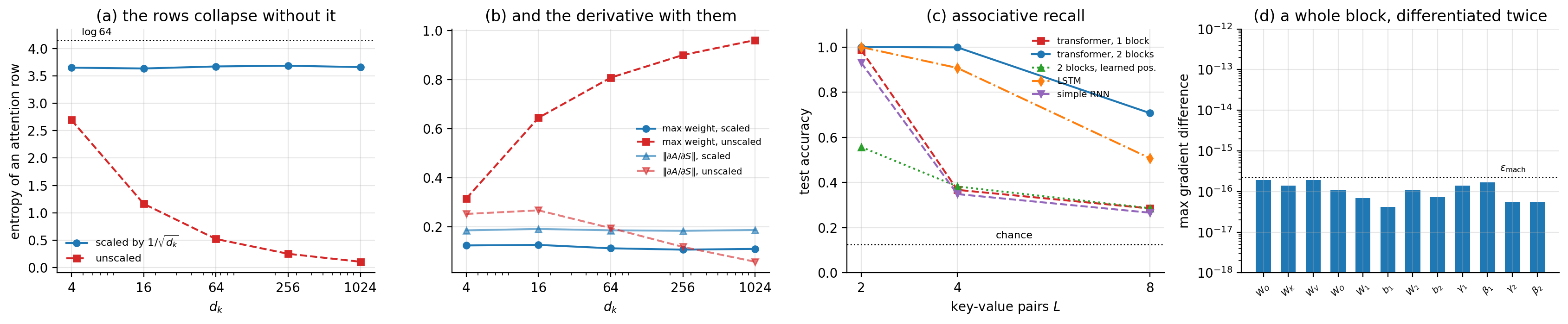
Figure 13.3: (a) The entropy of an attention row against \(d_k\), with and without the \(1/\sqrt{d_k}\) of Eq. (13.5), measured in PyTorch; the dashed line is \(\log 64\), the entropy of a uniform row. (b) The largest weight in a row and the norm of the softmax Jacobian: unscaled, the row becomes a hard maximum and the derivative disappears with it. (c) Associative recall, Table 13.2: one block fails where two succeed, and the learned positional encoding fails everywhere. (d) The largest disagreement between our gradients through a whole block and PyTorch’s, against the double-precision unit roundoff.
13.9. Strengths, weaknesses and what to remember#
A transformer replaces the fixed interaction patterns of the earlier architectures by couplings computed from the data, Eq. (13.16). Everything else – the multilayer perceptron, the residual connections, the normalisation – is machinery from earlier chapters, assembled to make that one idea trainable.
The properties are sharp and we proved them. Attention averages, so its output lies in the convex hull of its values (Proposition 13.1) and it cannot extrapolate without the feed-forward sublayer. It is equivariant to all permutations (Theorem 13.2), a much larger symmetry group than the translations of Theorem 10.7, which is why position has to be added by hand. It costs \(\bigO(n^{2}d)\) (Proposition 13.3), which is the price of global access and the reason for a large literature on approximating it.
The \(1/\sqrt{d_k}\) is not cosmetic. Proposition 13.4 predicts \(\var(\bm{q}\cdot\bm{k})=d_k\), measured as \(1011\) at \(d_k=1024\); and the softmax Jacobian falls by thirty-five orders of magnitude between logit scale \(1\) and scale \(64\). Without the scaling a wide head starts training with no usable gradient through its attention weights at all.
The result to carry away is Section What one attention layer cannot do. On associative recall at \(L=4\), a one-block transformer reached \(0.366\) and a matched recurrent network \(0.351\) – indistinguishable, and both far from the task. Two blocks reached \(0.993\). Seeing every position is not the same as being able to compose two retrievals, and depth here supplies steps of computation rather than capacity. Global access is necessary and not sufficient. Proposition 13.6 turns that observation into a statement with a proof: if keys and values depend on the symbol at their own position, no content-based score can single out the position after the match, because the symbol there is independent of the query. Repeating the whole table in PyTorch, Table 13.2, reproduces it to the third decimal – \(0.367\) against \(0.366\) for one block, \(0.999\) against \(0.993\) for two.
Two further things came out of running the libraries rather than reading them.
Proposition 13.5 shows the sinusoidal encoding to be an exactly
relative code, with translation acting on it as a fixed rotation,
Eq. (13.10); replacing it by a learned embedding and changing
nothing else drops recall from \(1.000\) to \(0.557\) at \(L=2\) and to chance at
\(L=8\), because the previous-token head that the induction mechanism needs is one
linear map on the sinusoidal code and a separate discovery at every position
without it. And our block, differentiated by autograd on NumPy, agrees
with PyTorch’s implementation of the same block to \(1.9\times10^{-16}\) on every
parameter array – softmax, layer normalisation and multi-head repacking
included.
Set against the strengths – global context, full parallelism across positions, excellent scaling with data and model size, a learned rather than assumed interaction structure – are real weaknesses: quadratic cost in sequence length, large data requirements, no inductive bias whatever about locality or order, and an interpretability that is better than a dense layer’s but far from complete. The architecture is a good default when the structure of the interactions is unknown and the data are plentiful. When the structure is known – locality in an image, causality in a time series, translation invariance in a homogeneous medium – a convolution or a recurrence encodes it for free, and free structure beats learned structure whenever the structure is right.
The programs are in the directory
doc/BookML/BookPrograms/chapter13_transformers.
Every listing above appears there as a numbered file, and three modules run start to finish and reproduce the numbers quoted in the text:
attention.py– scaled dot-product attention, multi-head attention, layer normalisation, the block of Eq. (13.14), causal masks, sinusoidal positional encodings, and batched versions of all of them.cross_check_attn.py– the three-way comparison of Section Do the three implementations agree?, with the head-packing conversions for both libraries written out.transformer_torch.py– the scaling measurement of Section The scaling, in the library, the permutation test of Section Permutation equivariance, tested and the recall table of Section Associative recall, in the frameworks.transformer_tf.py– the recall experiment in TensorFlow.verify_attention.py– row-stochasticity, the convex-hull property, permutation equivariance and its destruction by a mask, the logit-variance table, the softmax-saturation table, and the agreement between the looped and batched implementations.recall.pyandrun_recall.py– the associative-recall task of Table 13.1, with the one-block and two-block transformers and the Chapter 11 recurrent baseline.
The figures are generated by ch13_figures.py in
doc/BookML/BookFigures; neither is drawn by hand.
13.10. Exercises#
13.10.1. Warm-up exercises#
Shapes and costs. With \(n=512\), \(d=768\), \(H=12\) and \(d_k=d/H\): (a) what are the shapes of \(\bm{Q}\), \(\bm{K}\), \(\bm{V}\), \(\bm{A}\) and the output of one head? (b) How many parameters has one block with \(d_{\mathrm{ff}}=4d\), split between attention and the MLP? (c) How much memory does \(\bm{A}\) need in single precision, for all heads at once, and what happens at \(n=8192\)?
Permutation equivariance. Prove Theorem 13.2 for multi-head attention, and then show that adding the positional encoding of Eq. (13.9) destroys it. Is the composition equivariant to any group at all?
The convex hull. Verify Proposition 13.1 numerically, then construct a target output that a single attention layer provably cannot produce, and confirm that adding the MLP of Eq. (13.14) makes it reachable.
Temperature. Replace \(1/\sqrt{d_k}\) by \(\beta\) in Eq. (13.4) and study the limits \(\beta\to0\) and \(\beta\to\infty\). Show that the first gives uniform averaging and the second a hard \(\arg\max\), and relate both to Eq. (13.17). What is the entropy of the attention distribution in each limit?
Positional encodings. (a) Prove Proposition 13.5: exhibit the rotation \(\bm{R}_k\) of Eq. (13.10) and derive Eq. (13.11). (b) Plot \(\mathrm{PE}(m)\cdot\mathrm{PE}(m')\) against \(m-m'\) for \(d=64\) and confirm that all curves collapse onto one, as part (ii) requires. (c) The kernel is exactly relative but not monotonic in \(|m-m'|\). Find the first local maximum away from the origin and explain where it comes from. (d) Show that a learned positional embedding satisfies neither part of the proposition, and connect that to the third row of Table 13.2.
One layer is not enough. (a) Work through Proposition 13.6 and state precisely which hypothesis a second layer breaks. (b) Construct, by hand, weights for a two-layer model that solve the recall task exactly: a first layer that shifts by one using Eq. (13.10), and a second that matches on content. (c) Does the argument still apply if the value map is allowed to depend on position as well as on the symbol? If not, why does the one-block model in Table 13.2 still fail?
The scaling, empirically. Reproduce Section The scaling, in the library. (a) Confirm \(\var(\bm{q}\cdot\bm{k})=d_k\) over three decades. (b) Show that the softmax Jacobian \(\operatorname{diag}(\bm{a}) -\bm{a}\bm{a}^{\mathsf{T}}\) has Frobenius norm tending to zero as \(\bm{a}\) tends to a one-hot vector, and bound its spectral norm by \(1/4\). (c) Replace \(1/\sqrt{d_k}\) by \(1/d_k\) and by \(1\) and report the entropy at \(d_k=1024\) in each case. Which of the three is right, and why is it not a matter of taste?
Masks. Write the mask for (a) causal attention, (b) attention restricted to a window of width \(w\), (c) attention that ignores padding tokens. For (b), show that the layer becomes a convolution with a data-dependent kernel, and relate this to Theorem 10.2.
13.10.2. Project-style exercise: a transformer from scratch#
Part a: the machinery. Implement scaled dot-product attention, multi-head attention, layer normalisation and the block of Eq. (13.14). Verify row-stochasticity, the convex-hull property and permutation equivariance to machine precision, and check every gradient against finite differences. Implement the batched version and verify it against the looped one.
Part b: the scaling. Reproduce Proposition 13.4 and the saturation table of Section Why the \texorpdfstring{\(1/\sqrt{d_k}\)}{1/sqrt(dk)}. Then train the same model with and without the \(1/\sqrt{d_k}\) at several values of \(d_k\), and report at what \(d_k\) the unscaled version stops training at all. Plot the entropy of the attention distribution during training in both cases.
Part c: depth versus width. Reproduce Table 13.1. Then separate the two explanations for the one-block failure: is it depth, or capacity? Train a one-block model with the width increased until its parameter count matches the two-block model, and report what happens. Then extend the table to \(L=8\) and \(L=16\) and plot accuracy against \(L\) for one block, two blocks and the recurrent baseline.
Part d: reading the attention. For a trained two-block model, plot the attention matrices of both blocks on several test sequences. Can you identify the mechanism described in Section What one attention layer cannot do – one head copying the predecessor, another matching the query? Quantify it: measure how much of the first block’s attention mass sits on the diagonal offset by one.
Part e: against the alternatives. Compare the transformer, the convolutional network of Chapter 10 and the recurrent network of Chapter 11 on the same task at matched parameter counts, measuring accuracy, wall-clock time per update and memory. Then repeat on a task with genuinely local structure and report which architecture wins there. The two answers should differ, and the discussion of why is the point of the exercise.
Part f: a learned Green’s function. Solve the one-dimensional Poisson equation of Section The one-dimensional Poisson equation for many right-hand sides, and train an attention model to map the discretised source \(f(x_j)\) to the solution \(u(x_i)\), as in Eq. (13.21). Compare the learned attention matrix against the exact Green’s function of the operator. How close is it, and does it get closer with more data or with more blocks?
Part g: the cost. Measure the wall-clock time and peak memory of your attention implementation as \(n\) grows, and confirm Proposition 13.3. Then implement one approximation – a sliding window, a random sparse pattern, or a low-rank factorisation of \(\bm{A}\) – and report what it costs in accuracy on the recall task of part c.