
11. Chapter 11: Recurrent Neural Networks#
Chapter 10 restricted the dense layer of Chapter 8 by insisting that it respect the spatial structure of an image, and obtained convolution. This chapter makes the corresponding restriction for data with a temporal structure, and obtains recurrence.
The assumption being given up is a familiar one. Almost everything so far has supposed that the training examples are independent and identically distributed, and the bias-variance and resampling arguments of Chapter 2 lean on it heavily. For a sequence this is simply false: the value of a detector trace at one sample is strongly informative about the next, that is the entire content of the data, and a model that treats the samples as independent has thrown the signal away before it starts.
Sequences also break a structural assumption. A feed-forward network has a fixed input dimension; a convolutional network has a fixed input size too, up to the pooling that precedes its dense layers. Sequences come in different lengths, and we would like one model to handle all of them. A recurrent network does this by processing one element at a time and carrying a state forward, so that the same parameters serve a sequence of any length.
The material follows the lecture notes for weeks five to seven of FYS-STK3155/4155. We derive the architecture, derive backpropagation through time, prove the theorem that explains why long sequences are hard, measure the effect, and then examine the gated architectures that were invented to defeat it. As in Chapter 10, the from-scratch implementation is checked against PyTorch and TensorFlow with identical weights, so that the recursion of Eqs. (11.16)–(11.18) can be compared with what automatic differentiation actually produces; and the chapter closes with the experiment that the theory demands but the usual account omits – a task that a simple recurrent network provably cannot learn and a gated one can.
11.1. Sequences, and what we want from them#
Write \(x_{1:T}=(\bm{x}_1,\dots,\bm{x}_T)\) for a sequence of inputs. Three tasks cover most of what is asked of a sequence model:
that is, modelling the sequence itself, mapping a sequence to a sequence (filtering, forecasting), and mapping a sequence to a single label (classification, regime detection).
The first of these can always be factorised exactly, by the chain rule of probability,
Equation (11.2) is exact and useless as it stands, because the conditioning set grows without bound. What makes it tractable is the assumption that everything relevant in \(x_{1:t-1}\) can be summarised in a finite-dimensional state \(\bm{h}_t\), updated recursively:
This is a latent state-space model, and it should look familiar from physics: Eq. (11.3) is exactly the structure of a Markovian dynamical system, with \(f_\theta\) the update map and \(\bm{h}_t\) the state. The Kalman filter is the case in which \(f_\theta\) is linear and the noise Gaussian. A recurrent neural network is the case in which \(f_\theta\) and \(g_\theta\) are neural networks, so that the update map is learned rather than derived.
Ordered, correlated data of this kind is the norm rather than the exception in the physical sciences: detector readout streams and waveform traces, climate and seismic records, turbulence probes, molecular dynamics trajectories, spectroscopic scans, and state estimation in control and feedback. Sequential does not have to mean temporal – text and genomic sequences are ordered without carrying a time stamp – but our examples will be time series.
11.2. The architecture#
The simplest recurrent network, usually called the vanilla or simple RNN, realises Eq. (11.3) with one affine map and one activation. At each step \(t\),
with \(\bm{U}\in\mathbb{R}^{n_h\times n_x}\) mapping the input into the state, \(\bm{W}\in\mathbb{R}^{n_h\times n_h}\) mapping the state to itself, \(\bm{V}\in\mathbb{R}^{n_y\times n_h}\) reading the state out, and \(\bm{b}\), \(\bm{c}\) the biases. The hidden activation \(\sigma_h\) is almost always \(\tanh\), for reasons that Section Why long sequences are hard will make precise, and \(\sigma_y\) is the identity for regression or a softmax for classification. The recursion is started from \(\bm{h}^{(0)}=\bm{0}\) unless there is reason to do otherwise.
There are two equivalent ways of drawing Eq. (11.4), and Figure 11.1 shows both. On the left is the folded form: a single layer with an arrow leaving it and returning to itself, which is the literal content of the recursion and the reason for the name. On the right is the unrolled form, in which the same layer is drawn once per time step and the self-arrow becomes an arrow from one copy to the next. The two pictures describe the same computation. The folded one is how the network is stored – one copy of \(\bm{U},\bm{W},\bm{V}\) – and the unrolled one is how it is executed, and Section Backpropagation through time will show that the unrolled picture is also how it is differentiated.
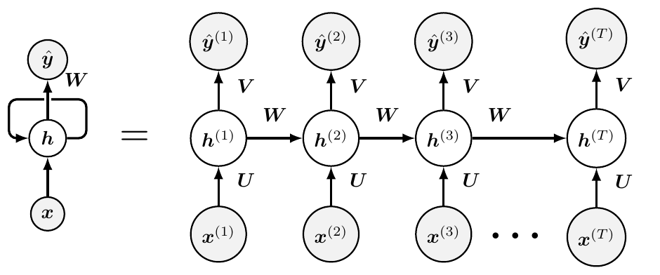
Figure 11.1: The recurrent network of Eq. (11.4), folded on the left and unrolled on the right. The input matrix \(\bm{U}\), the recurrent matrix \(\bm{W}\) and the output matrix \(\bm{V}\) are the same arrays at every step; the unrolled diagram repeats them but does not duplicate them. Unrolling turns the network into a feed-forward graph of depth \(T\) with tied weights, which is what makes backpropagation applicable and what makes Theorem 11.1 unavoidable.
Three properties of Eq. (11.4) are worth stating explicitly, because each is a deliberate design decision and each has a consequence.
The parameters do not depend on \(t\). The same \(\bm{U},\bm{W},\bm{V}\) act at every step. This is parameter sharing along the time axis, exactly analogous to the parameter sharing along the spatial axes that made a convolutional layer in Chapter 10, and it has the same two consequences: the parameter count is independent of the sequence length, and the model is equivariant to translation in time.
The state is a bottleneck. Everything the network will ever know about \(x_{1:t}\) when it computes \(\hat{\bm{y}}^{(t+1)}\) must fit in the \(n_h\) numbers of \(\bm{h}^{(t)}\). This is what makes the model tractable and also what limits it.
The cost accumulates over the sequence. For a regression task the cost is
and for classification \(L^{(t)}\) is the cross-entropy of Chapter 5. In the sequence-to-label case only \(L^{(T)}\) is non-zero, and Section Why long sequences are hard will show that this is the hardest case of all.
Parameter count
A simple RNN has \(n_h(n_x+n_h+1)+n_y(n_h+1)\) parameters, and the sequence length \(T\) appears nowhere. A feed-forward network given the same sequence flattened into a vector of length \(Tn_x\) would need \(\bigO(Tn_xn_h)\) weights in its first layer alone, and would have to be retrained for every new \(T\). This is the same argument as Eq. (10.1), transposed from space to time.
11.2.1. The RNN as a discrete-time dynamical system#
Set the input to zero, or hold it constant. Equation (11.4) becomes an autonomous map
and the entire vocabulary of dynamical systems applies. Fixed points satisfy \(\bm{h}^\star=F(\bm{h}^\star)\); their stability is decided by the eigenvalues of the Jacobian
with the fixed point attracting if the spectral radius \(\rho(\bm{J})<1\) and repelling if \(\rho(\bm{J})>1\). In more than one dimension the map can also possess limit cycles, and in three or more it can be chaotic.
This is not an idle observation. It tells us what a recurrent network is capable of representing – oscillations, decay to a point attractor, chaotic wandering – and it tells us what the network will do with information. If the dynamics are strongly contracting the network forgets its initial condition quickly and cannot carry information far; if they are expanding it is unstable. Equation (11.7) is also, as Section Why long sequences are hard will show, exactly the quantity that controls the gradient. The stability of the forward dynamics and the survival of the backward gradient are the same question.
11.3. Where the recurrence comes from: a differential equation#
The recurrence of Eq. (11.4) can look arbitrary. It is not, and the quickest way to see why is to derive it from a differential equation, which also connects this chapter to Chapter 9.
Take Newton’s equation for a damped harmonic oscillator, scaled so that time is dimensionless,
with \(\eta\) the damping and \(F\) an external force. As always we reduce it to two first-order equations by introducing the velocity,
Now discretise the velocity equation by the forward Euler method of Section Logistic population growth:
The right-hand side is a function of the current state and the current input. But \(v_i\) was itself produced by the same rule one step earlier,
so substituting gives
Absorbing the forcing into the input and renaming the output, this is
which is Eq. (11.3) exactly. A recurrent network is a learned, non-linear time-stepper. The hidden state plays the role of the integrator’s internal state, \(\bm{W}\) plays the role of \(1-\eta\Delta t\), and the training data supply what the differential equation would otherwise have to tell us.
The comparison with Chapter 9
Two chapters have now solved differential equations with networks, and they do it in opposite ways. In Chapter 9 the equation was known and supplied the cost through its residual; no data were needed and the network learned a function of continuous time. Here the equation is unknown and the data supply the cost; the network learns a discrete update rule. The first is appropriate when the physics is known and the data are absent, the second when the data are present and the physics is not.
11.4. Backpropagation through time#
Training uses gradient descent, so we need \(\nabla\mathcal{L}\). The standard way to see how is to unroll the recursion: a recurrent network run for \(T\) steps is a feed-forward network of depth \(T\) in which every layer shares the same weights. Backpropagation applies unchanged; the only novelty is that gradients from every step must be summed into the same parameter arrays.
The algorithm has a pleasing description in the time domain. The forward pass builds a stack of the activities at each step; the backward pass peels the activities off the stack, computing error derivatives at each step; and afterwards the derivatives at all steps are added together for each weight.
The output layer. Differentiating Eq. (11.5) gives, for each \(t\),
which for the quadratic cost and a linear \(\sigma_y\) is simply \((\hat{\bm{y}}^{(t)}-\bm{y}^{(t)})/T\).
The last hidden state. At \(t=T\) the state influences the cost only through the output at that step,
Earlier hidden states. For \(t<T\) the state has two routes to the cost: through the output at step \(t\), and through the state at step \(t+1\). The chain rule therefore gives two terms,
which, using Eq. (11.4), is
Equations (11.15) and (11.17) are run backwards from \(t=T\) to \(t=1\), and they are the whole of BPTT.
The parameters. Because the same matrices act at every step, each accumulates a contribution from every step:
where \(\bm{\delta}^{(t)}=\operatorname{diag}(\sigma_h'(\bm{a}^{(t)})) \nabla_{\bm{h}^{(t)}}\mathcal{L}\) is the error at the pre-activation of step \(t\).
The backward pass is linear
There is an asymmetry between the two passes that is easy to miss and important to notice. The forward pass is non-linear: the squashing function \(\sigma_h\) keeps the activities bounded, and this is what prevents them from exploding. The backward pass, by contrast, is completely linear in the incoming gradient – Eq. (11.16) is a matrix acting on \(\nabla_{\bm{h}^{(t+1)}}\mathcal{L}\), with the matrix fixed by the forward pass. Double the error at the final step and every error derivative doubles. Nothing bounds the backward pass, which is precisely why it can explode when the forward pass cannot.
11.5. Why long sequences are hard#
Iterating Eq. (11.17) from \(T\) back to \(t\) produces a product of Jacobians, one factor per step. It is this product, and not anything about the architecture as such, that makes recurrent networks hard to train.
Theorem 11.1 (Vanishing and exploding gradients)
Let \(\bm{h}^{(t)}=\sigma_h(\bm{U}\bm{x}^{(t)}+\bm{W}\bm{h}^{(t-1)}+\bm{b})\) and suppose \(|\sigma_h'(z)|\le\mu\) for all \(z\). Then for any \(t<T\)
and its spectral norm obeys
where \(\sigma_{\max}(\bm{W})\) is the largest singular value. Consequently, if \(\mu\,\sigma_{\max}(\bm{W})<1\) the gradient contribution from step \(t\) decays exponentially in the lag \(T-t\). If \(\mu\,\sigma_{\max}(\bm{W})>1\) it may grow exponentially.
Proof
Equation (11.19) is the chain rule applied to the recursion, one factor for each step, with \(\partial\bm{h}^{(k)}/\partial\bm{h}^{(k-1)} =\operatorname{diag}(\sigma_h'(\bm{a}^{(k)}))\bm{W}\) read off from Eq. (11.4). For the bound, the spectral norm is submultiplicative, so the norm of the product is at most the product of the norms. Each factor satisfies \(\|\operatorname{diag}(\sigma_h'(\bm{a}^{(k)}))\bm{W}\|_2 \le\|\operatorname{diag}(\sigma_h'(\bm{a}^{(k)}))\|_2\|\bm{W}\|_2 \le\mu\,\sigma_{\max}(\bm{W})\), since the spectral norm of a diagonal matrix is the largest absolute entry and that of \(\bm{W}\) is \(\sigma_{\max}(\bm{W})\). Multiplying \(T-t\) such bounds gives Eq. (11.20).
For \(\tanh\) we have \(\mu=1\), attained only at the origin, and for the logistic function \(\mu=1/4\), which is why \(\tanh\) is preferred: the logistic activation guarantees decay by a factor of at least four per step regardless of the weights. For ReLU, \(\mu=1\) as well, but the derivative is \(0\) or \(1\) rather than a number smoothly approaching \(1\), and a ReLU recurrent network is prone to explosion instead; this is why the rectified family, dominant everywhere else in this book, is largely absent from recurrent architectures.
Corollary 11.2 (Memory horizon)
If \(\mu\,\sigma_{\max}(\bm{W})<1\), define
Then Eq. (11.20) reads \(\|\partial\bm{h}^{(T)}/\partial\bm{h}^{(t)}\|_2\le e^{-(T-t)/\tau}\): the influence of step \(t\) on step \(T\) decays with a characteristic scale of \(\tau\) steps, and falls below a tolerance \(\varepsilon\) once \(T-t > \tau\log(1/\varepsilon)\).
Proof
Write \((\mu\sigma_{\max})^{T-t}=e^{(T-t)\log(\mu\sigma_{\max})}\) and substitute Eq. (11.21).
The number \(\tau\) deserves a name and a measurement, because it converts Theorem 11.1 from a qualitative warning into a design parameter: it is the length of sequence the network can actually use. We measure it in Section Measuring it, and the answer is smaller than one expects.
The bound is sufficient, not necessary
Equation (11.20) uses \(\sigma_{\max}(\bm{W})\), not the spectral radius \(\rho(\bm{W})\), and the two can differ substantially for non-normal \(\bm{W}\) – in the experiment below, \(\rho=0.5\) corresponds to \(\sigma_{\max}=0.85\) and \(\rho=1.5\) to \(\sigma_{\max}=2.56\). Since \(\rho(\bm{W})\le\sigma_{\max}(\bm{W})\) always, \(\mu\sigma_{\max}<1\) is a sufficient condition for the gradient to vanish, while \(\rho>1/\mu\) is necessary for sustained growth. Between the two lies a regime in which transient growth is possible even though the asymptotic behaviour is decay, and this is where carefully initialised recurrent networks actually operate.
11.5.1. Measuring it#
Theorem 11.1 is a bound; it is worth seeing the real thing. We take \(n_h=20\), sequences of length \(T=60\), and inputs small enough that the network stays near the origin where \(\tanh'\approx1\), so that the product is not confounded by saturation. We then form Eq. (11.19) explicitly and measure its spectral norm as a function of the lag, scaling \(\bm{W}\) so that its spectral radius takes prescribed values.
 rho(W)  sigma_max  mean max(tanh')   ||dh_T/dh_1||   bound sigma_max^59
  0.50     0.853        1.0000        1.683e-18        8.319e-05
  0.90     1.535        1.0000        3.487e-03        9.575e+10
  1.10     1.876        0.9999        3.751e+02        1.327e+16
  1.50     2.558        0.9882        2.998e+03        1.175e+24
At \(\rho(\bm{W})=0.5\) the influence of the first step on the last has fallen by eighteen orders of magnitude over fifty-nine steps. This is not a gradient that a floating-point optimiser can use; it is zero. At \(\rho(\bm{W})=1.1\) the same quantity has grown to \(375\), and at \(1.5\) to \(3000\), so that a single unlucky mini-batch can throw the parameters anywhere. The last column shows the bound (11.20) is satisfied and is very loose in the growing regime, as one would expect from a worst-case argument applied to a product of matrices whose singular vectors are not aligned.
Figure 11.2(a) plots the whole decay. The straight lines on the logarithmic axis are the exponential of Theorem 11.1, and the sign of the slope is decided by whether \(\rho(\bm{W})\) sits below or above one.
Because those lines are straight, Corollary 11.2 can be turned around: instead of bounding \(\tau\) from \(\sigma_{\max}(\bm{W})\), fit it to the measured decay. Doing so at every lag from \(1\) to \(59\) gives
=== 6. the memory horizon: fitted decay rate, Corollary 11.horizon ===
   rho(W)  sigma_max   fitted tau (steps)   lag for a factor 1e-6   norm at lag 59
    0.50     0.9129                 1.45                      20        1.967e-17
    0.70     1.2780                 2.82                      39        8.229e-09
    0.90     1.6431                 9.66                     133        2.264e-02
    1.10     2.0083               -10.30                    -142        3.116e+03
and this is the number to remember. At \(\rho(\bm{W})=0.5\) the memory horizon is one and a half steps. Not fifty, not ten: a network initialised this way has forgotten its input after two steps, and no amount of training on long sequences will change that until the weights themselves grow. At \(\rho=0.9\) the horizon reaches ten steps, which is still short against the \(T=60\) of the experiment, and by \(\rho=1.1\) the fitted \(\tau\) is negative – the product grows rather than decays, and the network is in the exploding regime. The useful range is narrow and it sits just below one.
Truncated backpropagation through time
Corollary 11.2 also licenses the standard economy. Running BPTT over a sequence of length \(T=10^{4}\) requires storing \(10^{4}\) activations; truncated BPTT propagates the gradient back only \(k\) steps and discards the rest. The error this introduces is exactly the discarded tail of Eq. (11.19), bounded by
so the bias falls exponentially in the truncation length with the same constant \(\tau\). Choosing \(k\) a few multiples of \(\tau\) makes the truncation error negligible against the gradient that survives – but note what this says: when \(\tau\) is small enough for truncation to be safe, the network has no long memory to lose, and when it has long memory, truncation destroys it. Truncated BPTT is cheap precisely when the recurrence is not doing the thing it was introduced for.
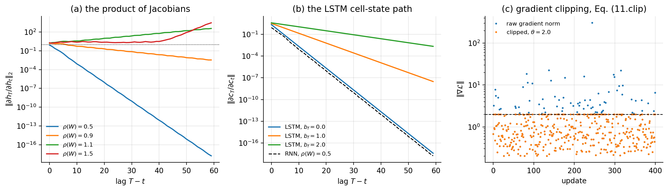
Figure 11.2: (a) The spectral norm of the Jacobian product (11.19) against the lag \(T-t\), for four values of the spectral radius of \(\bm{W}\). The exponential behaviour of Theorem 11.1 is the straight line on a logarithmic axis. (b) The same quantity for the cell state of an LSTM, Eq. (11.29), at three values of the forget-gate bias, with the \(\rho=0.5\) curve of panel (a) repeated as a dashed line. At \(b_f=0\) the LSTM is no better than the vanilla RNN; the advantage comes entirely from biasing the gate open. (c) Gradient clipping, Eq. (11.23): the rare large norms that would otherwise destroy the parameters are rescaled, the direction is kept and everything below the threshold is untouched.
11.5.2. Gradient clipping#
Vanishing and exploding gradients are not symmetric problems, and they do not have symmetric remedies. Explosion is the easier of the two, because it is visible: the gradient norm spikes and the parameters jump. The standard fix is to rescale any gradient whose norm exceeds a threshold, keeping the direction and discarding only the magnitude,
Two properties make Eq. (11.23) safe to apply unconditionally.
Proposition 11.3 (Clipping is a trust region and preserves descent)
Let \(\tilde{\bm{g}}\) be the clipped gradient of Eq. (11.23). Then (i) \(\tilde{\bm{g}}=\lambda\bm{g}\) with \(\lambda=\min(1,\theta/\|\bm{g}\|) \in(0,1]\), so \(\langle\tilde{\bm{g}},\bm{g}\rangle=\lambda\|\bm{g}\|^{2}>0\) whenever \(\bm{g}\neq\bm{0}\) and \(-\tilde{\bm{g}}\) is a descent direction; (ii) \(\tilde{\bm{g}}\) is the solution of
that is, the Euclidean projection of \(\bm{g}\) onto the ball of radius \(\theta\); so a step of size \(\gamma\) on the clipped gradient never moves the parameters further than \(\gamma\theta\).
Proof
(i) is immediate from the definition, since \(\lambda>0\) in both branches. For (ii), the projection of \(\bm{g}\) onto \(\{\|\bm{u}\|\le\theta\}\) minimises \(\|\bm{u}-\bm{g}\|^{2}\); writing \(\bm{u}=r\hat{\bm{u}}\) with \(r\le\theta\) gives \(\|\bm{u}-\bm{g}\|^{2}=r^{2}-2r\langle\hat{\bm{u}},\bm{g}\rangle+\|\bm{g}\|^{2}\), minimised over directions at \(\hat{\bm{u}}=\bm{g}/\|\bm{g}\|\) and then over \(r\) at \(r=\min(\|\bm{g}\|,\theta)\).
The two statements are why clipping is not a hack. Property (i) says the optimiser is still doing gradient descent, on a rescaled gradient; property (ii) says the effective step length is bounded by \(\gamma\theta\) regardless of what the loss surface does, which is exactly the guarantee a trust-region method provides. What is lost is scale information: near a genuine cliff the clipped step is far shorter than the true gradient suggests, so progress is slow rather than catastrophic. That is the intended trade. This is not a descent direction for any modified cost and it has no convergence theory worth the name, but it is close to universal in practice and it is essentially free. Figure 11.2(c) shows the effect: the bulk of the updates are untouched and only the rare spikes are cut. Note that clipping does nothing whatever for vanishing gradients – rescaling a gradient of \(10^{-18}\) upwards would amplify rounding noise, not signal. Vanishing gradients require a change of architecture, which is the subject of Section Long short-term memory.
Careful initialisation helps with both. Setting \(\sigma_{\max}(\bm{W})\approx1\) puts the network at the edge between the two regimes, which is the best one can do with this architecture; the orthogonal or identity initialisations sometimes used for recurrent weights are attempts to sit exactly there.
11.6. Implementation and verification#
As in Chapters 8 and 10 we write the network from scratch and check the gradients before trusting anything.
def forward(p, X, h0=None):
    """X has shape (T, n_in).  Returns outputs (T, n_out) and the cache.

    a_t = U x_t + W h_{t-1} + b,   h_t = tanh(a_t),   yhat_t = V h_t + c
    """
    T = X.shape[0]
    n_h = p["W"].shape[0]
    H = np.zeros((T + 1, n_h))              # H[0] is h_{-1}
    if h0 is not None:
        H[0] = h0
    A = np.zeros((T, n_h))
    Y = np.zeros((T, p["V"].shape[0]))
    for t in range(T):
        A[t] = p["U"] @ X[t] + p["W"] @ H[t] + p["b"]
        H[t + 1] = np.tanh(A[t])
        Y[t] = p["V"] @ H[t + 1] + p["c"]
    return Y, (X, A, H)
The backward pass is Eqs. (11.15)–(11.18), read off line by line. Note the single loop running backwards and the accumulation with \verb!+=! into arrays that were zeroed once: that accumulation is the weight sharing.
def bptt(p, cache, Y, target, return_norms=False):
    """Gradients of Eq. (11.cost) by the recursion (11.bptth)."""
    X, A, H = cache
    T = X.shape[0]
    g = {k: np.zeros_like(v) for k, v in p.items()}
    dY = (Y - target) / T                    # dL/dyhat_t for the cost (11.cost)
    dh_next = np.zeros(p["W"].shape[0])
    norms = []
    for t in reversed(range(T)):
        g["V"] += np.outer(dY[t], H[t + 1])
        g["c"] += dY[t]
        dh = p["V"].T @ dY[t] + dh_next      # Eq. (11.bptth)
        da = (1.0 - H[t + 1] ** 2) * dh      # through tanh
        g["U"] += np.outer(da, X[t])
        g["W"] += np.outer(da, H[t])
        g["b"] += da
        dh_next = p["W"].T @ da
        if return_norms:
            norms.append(np.linalg.norm(dh))
    return (g, norms[::-1]) if return_norms else g
Clipping is Eq. (11.23) applied to all parameter arrays jointly, since it is the norm of the full gradient vector that matters:
def clip(g, theta):
    """Rescale the whole gradient if its norm exceeds theta."""
    n = np.sqrt(sum(np.sum(v ** 2) for v in g.values()))
    if n > theta:
        for k in g:
            g[k] *= theta / n
    return g, n
Checking against central differences over every entry of every parameter array, for a sequence of length twelve:
--- BPTT vs central differences (T=12) ---
  U: max relative error over all 12 entries = 1.38e-09
  W: max relative error over all 36 entries = 3.22e-08
  V: max relative error over all 6 entries = 1.53e-09
  b: max relative error over all 6 entries = 8.25e-10
  c: max relative error over all 1 entries = 1.41e-10
Unlike the convolutional network of Chapter 10, this check passes everywhere without a smooth surrogate, because \(\tanh\) and the quadratic cost are differentiable everywhere and there is no max-pooling argmax to switch.
11.6.1. The damped oscillator#
We test the network on the problem of Section Where the recurrence comes from: a differential equation. A fourth-order Runge-Kutta integrator generates the trajectory of Eq. (11.8) with \(\eta=0.2\) over \(t\in[0,40]\) at \(800\) points, and the network is trained by BPTT with clipping at \(\theta=1\) to predict \(x_{i+1}\) from \(x_i\) along sequences of length \(40\). The training data come from a single trajectory, with initial condition \((x_0,v_0)=(1,0)\) and no forcing. We then test on data the network has never seen:
train, IC (1,0)            MSE 2.275e-05   Var(x)=0.0655  rel 0.035%
test, unseen IC (0,1)      MSE 2.218e-05   Var(x)=0.0618  rel 0.036%
test, driven+unseen IC     MSE 3.595e-05   Var(x)=0.1488  rel 0.024%
The second line is the interesting one. The network was trained on a trajectory starting from rest at unit displacement, and tested on one starting from the origin at unit velocity – a different solution of the same equation, out of phase with everything it saw – and the error is identical to the training error, three parts in ten thousand of the variance. The third line goes further: an oscillator driven by \(F(t)=0.3\cos(0.7t)\), which the network never saw in any form, is predicted just as well.
The network has therefore not memorised a trajectory; it has learned the update rule, which is what Eq. (11.12) said it would do. That is the payoff of the recurrent structure, and it is the same payoff parameter sharing gave in Chapter 10: a rule learned once applies everywhere it is valid.
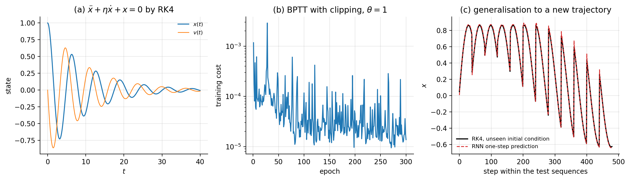
Figure 11.3: (a) The damped oscillator (11.8) with \(\eta=0.2\), integrated by fourth-order Runge-Kutta; the network sees only \(x(t)\). (b) The training cost under BPTT with clipping at \(\theta=1\). (c) One-step predictions on a trajectory with an initial condition the network never saw, against the Runge-Kutta solution.
11.7. Long short-term memory#
Theorem 11.1 says that the trouble comes from a product of Jacobians, each carrying a factor of \(\bm{W}\) and a factor of \(\sigma_h'\). Any architecture that keeps the gradient alive over long lags must break that product. The long short-term memory unit of Hochreiter and Schmidhuber [hochreiter1997] does so by introducing a second state variable whose update is additive rather than multiplicative.
The design is usually described as a memory cell with gates. A linear unit with a self-connection of weight one maintains its value indefinitely; information is written into it when a write gate opens, kept while a keep gate is open, and read out when a read gate opens. Because the gates are logistic functions they are differentiable, so the whole circuit can be trained by backpropagation. In modern notation the three gates are called the input, forget and output gates, and the cell carries a long-term state \(\bm{c}\) alongside the short-term state \(\bm{h}\).
The forget gate. decides how much of the existing cell state to retain:
The logistic \(\sigma\) returns values near \(0\) for very negative arguments and near \(1\) for very positive ones, so \(\bm{f}^{(t)}\) acts as a soft, learned, per-component switch on the long-term memory.
The input gate. decides what to write, and is two functions rather than one: a logistic deciding how much to write and a \(\tanh\) deciding what,
The cell update. combines the two, with \(\odot\) the elementwise product:
The output gate. decides how much of the cell to expose as the visible state:
The unit has four times the parameters of a simple RNN with the same \(n_h\), since each of \(\bm{f},\bm{i},\bm{g},\bm{o}\) has its own \(\bm{W}_{\cdot x}\), \(\bm{W}_{\cdot h}\) and bias.
Figure 11.4 assembles the four equations into the circuit they describe. It repays a slow reading, because the geometry is the argument. Follow the horizontal line at the top, entering as \(\bm{c}^{(t-1)}\) and leaving as \(\bm{c}^{(t)}\): along the way it is multiplied once, by the forget gate, and added to once, by the input gate. That is all. It passes through no weight matrix and no squashing function, which is precisely why Eq. (11.29) contains neither. Every other path in the diagram – the four gates along the bottom, the output multiplication on the right – hangs off that line rather than lying on it.
Contrast the same picture for the simple RNN, which would have the state line running through a matrix multiplication and a \(\tanh\) at every step. The LSTM did not remove those operations; it moved them off the memory path.
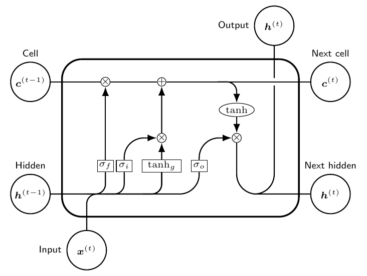
Figure 11.4: The LSTM cell of Eqs. (11.25)–(11.28). The four boxes along the bottom are the gates: \(\sigma_f\) the forget gate, \(\sigma_i\) and \(\tanh_g\) the two halves of the input gate, and \(\sigma_o\) the output gate, each taking \(\bm{x}^{(t)}\) and \(\bm{h}^{(t-1)}\) and each with its own weights. The circled \(\times\) and \(+\) are elementwise product and sum. The horizontal line carrying \(\bm{c}^{(t-1)}\) to \(\bm{c}^{(t)}\) is the constant error carousel: it meets one multiplication and one addition and no weight matrix, which is the content of Eq. (11.29) and the reason gradients survive along it.
11.7.1. Why it works, and by how much#
The point of Eq. (11.27) is what it does to the Jacobian. Differentiating the cell update with respect to the previous cell state, and treating the gates as slowly varying,
Compare with Eq. (11.19). There is no \(\bm{W}\) and no \(\sigma_h'\); the product is over the forget gates alone. If the network learns to hold \(\bm{f}^{(k)}\approx1\) on some component, the gradient along that component is transmitted essentially undamped for as long as the gate stays open. This is often called the constant error carousel, and it is the whole idea.
That is the argument. It is worth checking, because the argument is often stated as though the LSTM simply solves the problem, and it does not. Measuring Eq. (11.29) on an untrained LSTM with \(n_h=20\) and \(T=60\), for three values of the forget-gate bias:
  forget bias 0.0: mean f=0.5000  ||dc_T/dc_1||=3.879e-18
  forget bias 1.0: mean f=0.7311  ||dc_T/dc_1||=3.074e-08
  forget bias 2.0: mean f=0.8810  ||dc_T/dc_1||=2.232e-03
against \(1.683\times10^{-18}\) for the vanilla RNN at \(\rho(\bm{W})=0.5\). With \(\bm{b}_f=0\) the forget gates sit at \(\sigma(0)=1/2\), the product is \(2^{-59}\approx10^{-18}\), and the LSTM is no better than the simple RNN it was invented to replace. The gain is entirely a matter of where the gates start: biasing them open moves the mean gate to \(0.73\) and buys ten orders of magnitude, and a bias of two buys fifteen. Figure 11.2(b) shows the three curves with the vanilla RNN underneath, and the \(b_f=0\) curve lies almost exactly on top of it.
Initialise the forget-gate bias positive
This is the practical consequence, and it is why implementations commonly default to \(\bm{b}_f=1\); the empirical survey of Jozefowicz et al. [jozefowicz2015] found it to be among the most reliable single adjustments to recurrent training. The architecture supplies a path along which gradients can travel undamped; the initialisation decides whether the network starts anywhere near it. This is the same lesson as the He and Xavier initialisations of Chapter 8, in a setting where the consequence is measured in orders of magnitude rather than factors.
Equation (11.29) is approximate, and it is worth writing the exact statement, because what the approximation drops is not negligible.
Proposition 11.4 (The exact cell Jacobian)
With the gates of Eqs. (11.25)–(11.28),
where, writing \(\bm{D}_f=\operatorname{diag}(\bm{f}(1-\bm{f}))\), \(\bm{D}_i=\operatorname{diag}(\bm{i}(1-\bm{i}))\), \(\bm{D}_g=\operatorname{diag}(1-\bm{g}^{2})\) for the gate derivatives at step \(t\),
Proof
Differentiate Eq. (11.27). The explicit dependence on \(\bm{c}^{(t-1)}\) gives \(\operatorname{diag}(\bm{f}^{(t)})\). The remaining dependence is through \(\bm{h}^{(t-1)}=\bm{o}^{(t-1)}\odot\tanh\bm{c}^{(t-1)}\), which enters \(\bm{f}^{(t)},\bm{i}^{(t)},\bm{g}^{(t)}\) through \(\bm{W}_{fh},\bm{W}_{ih},\bm{W}_{gh}\); the chain rule with the elementwise derivatives \(\bm{D}_f,\bm{D}_i,\bm{D}_g\) gives the bracket, and \(\partial\bm{h}^{(t-1)}/\partial\bm{c}^{(t-1)} =\operatorname{diag}(\bm{o}^{(t-1)}(1-\tanh^{2}\bm{c}^{(t-1)}))\) is the final factor. Note that \(\bm{o}^{(t-1)}\) depends on \(\bm{h}^{(t-2)}\), not on \(\bm{c}^{(t-1)}\), so the expression closes.
Every term of \(\bm{R}^{(t)}\) carries a logistic derivative, bounded by \(1/4\), and the factor \(1-\tanh^{2}\bm{c}^{(t-1)}\), which vanishes as the cell state saturates. One would therefore expect \(\bm{R}\) to be negligible in the regime the architecture is designed for. Measuring it – assembling \(\partial\bm{c}^{(T)}/\partial\bm{c}^{(1)}\) exactly by automatic differentiation and comparing against the product of forget gates alone – shows that this expectation is wrong:
=== 5. Eq. (11.lstmjac) is approximate: how approximate? ===
  input scale   b_f   mean f   prod diag(f)   exact ||dc_T/dc_1||   ratio
          1.0   0.0   0.5185       1.891e-11             2.255e-08   1192.07
          1.0   1.0   0.7284       2.538e-05             1.514e-03     59.63
          1.0   2.0   0.8693       1.808e-02             5.654e-01     31.27
          1.0   4.0   0.9759       5.970e-01             8.408e+00     14.08
          0.1   0.0   0.5007       2.672e-12             4.828e-07   180716.73
          0.1   1.0   0.7310       6.201e-06             7.472e-02   12048.86
          0.1   2.0   0.8799       1.247e-02             8.597e+00    689.13
          0.1   4.0   0.9789       5.848e-01             1.144e+02    195.66
The ratio never approaches one. Biasing the gates open improves it by two orders of magnitude, from \(1192\) to \(14\); driving the cell more gently makes it far worse, because a cell state near zero has \(1-\tanh^{2}\bm{c}\approx1\) and the gate paths of Eq. (11.31) are then at their most conductive. So Eq. (11.29) should be read as a lower bound on how much gradient survives, not as an estimate of it.
The sign of the discrepancy is favourable: the true Jacobian is larger than the constant-error-carousel argument promises, so the LSTM transmits more gradient than the standard story claims, by one to five orders of magnitude in these measurements. But the standard story is not quantitative, and it is worth knowing that the gates are not merely a valve on a passive channel – they are themselves a conducting path.
One further point. Nothing here prevents explosion: since \(\bm{f}\le\bm{1}\) the diagonal term of Eq. (11.30) cannot amplify, but \(\bm{R}^{(t)}\) contains weight matrices with no such bound, so clipping remains necessary.
11.7.2. The gated recurrent unit#
The gated recurrent unit of Cho et al. [cho2014] applies the same idea with fewer parts. It drops the separate cell state, keeping only \(\bm{h}\), and uses two gates instead of three:
The update gate \(\bm{z}\) plays the roles of both the forget and input gates at once – what is not written is retained, by construction – and the reset gate \(\bm{r}\) controls how much of the past enters the candidate state. The last line has the same additive form as Eq. (11.27), so the same constant-error-carousel argument applies with \(1-\bm{z}\) in place of \(\bm{f}\).
A GRU has three sets of weight matrices against the LSTM’s four, so about three quarters of the parameters and correspondingly less computation. Which performs better is task-dependent and not settled; the two are usually close. More recent work continues in the same direction: Beck et al. [beck2024] report that exponential gating and modified memory structures make an extended LSTM competitive with transformers and state-space models in both performance and scaling.
11.8. The same networks in PyTorch and TensorFlow#
Everything so far has been derived and then implemented in NumPy. This section hands the same architectures to the two libraries, and does three things with them: runs the two standard examples, checks that the libraries and our code compute the same function to rounding, and then asks the question the theory has been building towards – whether the gating of Section Long short-term memory lets a network learn something a simple recurrent network cannot.
11.8.1. Forecasting a sine wave#
The task is the one-step-ahead forecasting of Section The damped oscillator, on a sine wave rather than a damped oscillator. Sequences of \(20\) consecutive values are used to predict the next.
import numpy as np
import tensorflow as tf

# 1. Data: a sine wave cut into overlapping windows
time_steps = np.linspace(0, 100, 500)
data = np.sin(time_steps)
seq_length = 20
X, y = [], []
for i in range(len(data) - seq_length):
    X.append(data[i:i+seq_length])
    y.append(data[i+seq_length])
X = np.array(X).reshape(-1, seq_length, 1)     # (samples, timesteps, features)
y = np.array(y).reshape(-1, 1)

split = int(0.8 * len(X))
X_train, X_test = X[:split], X[split:]
y_train, y_test = y[:split], y[split:]

# 2. Model: a SimpleRNN layer is exactly Eq. (11.rnn)
model = tf.keras.Sequential([
    tf.keras.layers.SimpleRNN(16, input_shape=(seq_length, 1)),
    tf.keras.layers.Dense(1),
])
model.compile(optimizer="adam", loss="mse")
model.summary()      # 16*(1+16+1) = 288 recurrent parameters, then 17

# 3. Training and evaluation
history = model.fit(X_train, y_train, epochs=50, batch_size=32,
                    validation_split=0.2, verbose=1)
print(f"test loss {model.evaluate(X_test, y_test, verbose=0):.4f}")
The same in PyTorch, where the loop is explicit:
import numpy as np
import torch
import torch.nn as nn

seq_length = 20
data = np.sin(np.linspace(0, 100, 500)).astype("float32")
X = np.stack([data[i:i+seq_length] for i in range(len(data)-seq_length)])
y = data[seq_length:].reshape(-1, 1)
X = torch.tensor(X).unsqueeze(-1)              # (N, T, 1), batch_first
y = torch.tensor(y)
split = int(0.8 * len(X))


class SineRNN(nn.Module):
    """nn.RNN implements Eq. (11.rnn) with tanh by default."""
    def __init__(self, hidden=16):
        super().__init__()
        self.rnn = nn.RNN(input_size=1, hidden_size=hidden, batch_first=True)
        self.fc = nn.Linear(hidden, 1)

    def forward(self, x):
        out, h_T = self.rnn(x)                 # out: (N, T, hidden)
        return self.fc(out[:, -1, :])          # read out the last state only


model = SineRNN()
opt = torch.optim.Adam(model.parameters(), lr=1e-3)
lossfn = nn.MSELoss()
for epoch in range(50):
    model.train()
    opt.zero_grad()
    loss = lossfn(model(X[:split]), y[:split])
    loss.backward()                            # BPTT, Eqs. (11.bptth)-(11.bpttparams)
    nn.utils.clip_grad_norm_(model.parameters(), 1.0)   # Eq. (11.clip)
    opt.step()
    if (epoch + 1) % 10 == 0:
        print(f"epoch {epoch+1}: train loss {loss.item():.5f}")

model.eval()
with torch.no_grad():
    print(f"test loss {lossfn(model(X[split:]), y[split:]).item():.5f}")
Note \verb!clip_grad_norm_!, which is Eq. (11.23) exactly and is justified by Proposition 11.3, and the line \verb!out[:, -1, :]!, which selects the sequence-to-label case of Eq. (11.1): only the final state is read.
Run for two hundred epochs with minibatches of thirty-two, both reach the same place:
PyTorch    epoch 200: train mse 0.000008   test mse 0.000004   (321 parameters)
TensorFlow epoch 200: train mse 0.000003   test mse 0.000002   (305 parameters)
A test mean squared error of \(4\times10^{-6}\) is a root-mean-square error of \(0.003\) on a signal of unit amplitude, and Figure 11.5(a) shows the two predictions lying on the true curve. The parameter counts differ by sixteen, and the reason is the convention noted below: PyTorch’s \verb!nn.RNN! carries two bias vectors where Eq. (11.4) and Keras carry one. Their sum is our \(\bm{b}\), so the models are the same; only the parameterisation is redundant.
11.8.2. An LSTM on MNIST, read row by row#
A less obvious use is to treat each \(28\times28\) image as a sequence of \(28\) rows, each of \(28\) features, and classify it with an LSTM. This is not what one would do in practice – Chapter 10 explains why a convolutional network is the right tool for images – but it is a clean demonstration of a sequence-to-label task, and comparing it against Section Does it actually help? An experiment is instructive.
import tensorflow as tf
from tensorflow.keras.models import Sequential
from tensorflow.keras.layers import LSTM, Dense
from tensorflow.keras.utils import to_categorical

(x_train, y_train), (x_test, y_test) = tf.keras.datasets.mnist.load_data()
x_train = x_train.astype("float32") / 255.0
x_test = x_test.astype("float32") / 255.0
x_train = x_train.reshape((-1, 28, 28))        # 28 timesteps of 28 features
x_test = x_test.reshape((-1, 28, 28))
y_train = to_categorical(y_train, 10)
y_test = to_categorical(y_test, 10)

model = Sequential([
    LSTM(128, input_shape=(28, 28)),           # 4*128*(28+128+1) = 80384 params
    Dense(10, activation="softmax"),
])
model.compile(loss="categorical_crossentropy", optimizer="adam",
              metrics=["accuracy"])
model.summary()
model.fit(x_train, y_train, batch_size=64, epochs=10, validation_split=0.2)
test_loss, test_acc = model.evaluate(x_test, y_test, verbose=2)
print(f"test accuracy {test_acc:.4f}")
and in PyTorch:
import torch
import torch.nn as nn
from torchvision import datasets, transforms
from torch.utils.data import DataLoader

device = torch.device("cuda" if torch.cuda.is_available() else "cpu")
transform = transforms.Compose([transforms.ToTensor(),
                                transforms.Normalize((0.1307,), (0.3081,))])
train_loader = DataLoader(datasets.MNIST("./data", train=True, download=True,
                                         transform=transform),
                          batch_size=64, shuffle=True)
test_loader = DataLoader(datasets.MNIST("./data", train=False,
                                        transform=transform), batch_size=64)


class LSTMModel(nn.Module):
    """Eqs. (11.lstmf)-(11.lstmh); nn.LSTM already biases b_f, see below."""
    def __init__(self, input_size=28, hidden_size=128, num_classes=10):
        super().__init__()
        self.lstm = nn.LSTM(input_size, hidden_size, batch_first=True)
        self.fc = nn.Linear(hidden_size, num_classes)

    def forward(self, x):
        x = x.reshape(-1, 28, 28)              # image as a sequence of rows
        out, _ = self.lstm(x)                  # (batch, seq, hidden)
        return self.fc(out[:, -1, :])          # last state -> class scores


model = LSTMModel().to(device)
criterion = nn.CrossEntropyLoss()
optimizer = torch.optim.Adam(model.parameters(), lr=1e-3)

for epoch in range(10):
    model.train()
    for images, labels in train_loader:
        images, labels = images.to(device), labels.to(device)
        optimizer.zero_grad()
        loss = criterion(model(images), labels)
        loss.backward()
        nn.utils.clip_grad_norm_(model.parameters(), 1.0)
        optimizer.step()
    model.eval()
    correct = total = 0
    with torch.no_grad():
        for images, labels in test_loader:
            pred = model(images.to(device)).argmax(dim=1)
            correct += (pred == labels.to(device)).sum().item()
            total += labels.size(0)
    print(f"epoch {epoch+1}: test accuracy {100*correct/total:.2f}%")
Two remarks. PyTorch’s \verb!nn.LSTM! does not initialise the forget-gate bias to one; it draws all biases uniformly from \((-1/\sqrt{n_h},1/\sqrt{n_h})\), so the mean forget gate starts at about \(0.5\) – which by Section Why it works, and by how much is the worst case. Setting it explicitly is a few lines and is worth doing for long sequences. And the parameter count \(4n_h(n_x+n_h+1)\) printed by \verb!model.summary()! is a useful check of the four gates of Eqs. (11.25)–(11.28); if the number is not four times that of a simple RNN, something is wrong.
11.8.3. Do the three implementations agree?#
The listings and the NumPy code of Section Implementation and verification are supposed to be the same function, and the recurrent case has more room for disagreement than the convolutional one of Section Do the three implementations agree?, because three conventions differ at once:
PyTorch’s \verb!nn.RNN! and \verb!nn.LSTM! carry two bias vectors, \verb!bias_ih! and \verb!bias_hh!, where Eq. (11.4) has one. Their sum is our \(\bm{b}\).
Keras stores the input matrix transposed – \verb!kernel! of shape \((n_x,n_h)\) against our \(\bm{U}\) of shape \((n_h,n_x)\) – and likewise the recurrent matrix.
Both concatenate the four LSTM gates into one array in the order \((\bm{i},\bm{f},\bm{g},\bm{o})\), whereas Eqs. (11.25)–(11.28) introduce them as \((\bm{f},\bm{i},\bm{g},\bm{o})\). Getting this wrong produces a network that trains perfectly well and is not the one on the page.
With those reconciled, one set of weights in all three:
=== 1. the simple RNN of Eq. (11.rnn), forward ===
  hidden states  max |ours - torch| : 2.220e-16
  hidden states  max |ours - keras| : 4.441e-16
  outputs        max |ours - torch| : 2.220e-16
  outputs        max |ours - keras| : 3.331e-16

=== 2. backpropagation through time, Eqs. (11.bptth)-(11.bpttparams) ===
  our loss, Eq. (11.cost)   : 1.171647902250
  torch loss                : 1.171647902250
   array   shape        |ours - torch|      scale
   U     (8, 3)            5.551e-17   2.105e-01
   W     (8, 8)            5.551e-17   2.329e-01
   V     (2, 8)            1.110e-16   2.509e-01
   b     (8,)              1.110e-16   2.766e-01
   c     (2,)              1.110e-16   6.103e-01

=== 3. the LSTM cell, Eqs. (11.lstmf)-(11.lstmh) ===
  cell output    max |ours - torch| : 8.327e-17
  cell output    max |ours - keras| : 1.388e-16
Every entry is at unit roundoff; Figure 11.5(d) plots the backward-pass comparison. The recursion of Eqs. (11.15)–(11.18), derived by hand in Section Backpropagation through time, is what reverse-mode automatic differentiation computes.
The same idea settles Theorem 11.1. Rather than forming the product of Eq. (11.19) ourselves, we can ask autograd for \(\partial\bm{h}^{(T)}/\partial\bm{h}^{(1)}\) column by column, with no reference to the theorem at all:
=== 4. Theorem 11.vanishing, measured by autograd in PyTorch ===
   rho(W)   ||dh_T/dh_1|| autograd   ||dh_T/dh_1|| Eq. (11.jacprod)   ratio
    0.50                1.967e-17                   1.967e-17    1.0000
    0.90                2.264e-02                   2.264e-02    1.0000
    1.10                3.116e+03                   3.116e+03    1.0000
    1.50                7.351e+04                   7.351e+04    1.0000
The vanishing gradient is not an artefact of our implementation, and it is not something a better library avoids. It is a property of the composition.
11.8.4. Row by row: the two libraries on MNIST#
Training the LSTM of the listing above, and a simple RNN of the same width for comparison, for three epochs on the full sixty thousand images:
\noalign{} Cell |
Framework |
Parameters |
Test accuracy |
Seconds/epoch |
|---|---|---|---|---|
\noalign{}\noalign{} LSTM |
PyTorch |
\(82\,186\) |
\(0.9708\) |
\(8\) |
LSTM |
TensorFlow |
\(81\,674\) |
\(0.9743\) |
\(21\) |
simple RNN |
PyTorch |
\(21\,514\) |
\(0.9333\) |
\(6\) |
simple RNN |
TensorFlow |
\(21\,386\) |
\(0.9623\) |
\(7\) |
\noalign{} |
Table 11.1: MNIST read as \(28\) rows of \(28\), after three epochs with Adam at \(10^{-3}\) and batches of \(64\). Both cells have \(n_h=128\); the LSTM has four gates and therefore about four times the parameters. Compare the convolutional network of Section Training on MNIST, and what the dense layer is worth, which reaches \(0.99\) on the same data.
Three things are worth reading off Table 11.1. The LSTM beats the simple RNN, by three points in PyTorch and one in TensorFlow, on a task with only \(28\) time steps – short enough that Corollary 11.2 does not forbid the simple RNN from working, and it does work, just less well. The parameter counts differ between frameworks by exactly \(4n_h\) and \(n_h\), the extra bias vector again. And the whole exercise reaches \(0.97\) where the convolutional network of Section Training on MNIST, and what the dense layer is worth reached \(0.99\) with a comparable budget: reading an image as a sequence throws away the vertical structure that Chapter 10 was built to exploit, and the cost of doing so is visible.
11.8.5. The experiment the theory demands#
Section Why it works, and by how much showed that the LSTM keeps a larger Jacobian than a simple RNN, and Table 11.1 showed it classifying slightly better over \(28\) steps. Neither is the claim the architecture was invented to support, which is that gating lets a network learn dependencies a simple recurrence cannot. Testing that needs a task where nothing but long-range memory is being measured.
The standard one is the adding problem. Each sequence has two channels: the first carries values drawn uniformly from \([0,1]\), the second is zero except for exactly two markers, one in each half of the sequence. The target is half the sum of the two marked values. Nothing can be inferred from the local statistics – the values are independent and identically distributed – so a model must hold one number from the first half of the sequence until the second marker arrives, while ignoring everything in between. Predicting the mean and stopping gives a mean squared error of about \(0.043\), and that is the number to beat.
=== 3. the adding problem at increasing sequence length ===
   T   baseline         rnn        lstm         gru
    10    0.0427      0.0016      0.0000      0.0000
    30    0.0429      0.0411      0.0001      0.0000
    60    0.0411      0.0407      0.0002      0.0001
   120    0.0425      0.0427      0.0006      0.0001
This is the cleanest result in the chapter. At \(T=10\) the simple recurrent network solves the task, reaching \(0.0016\) against a baseline of \(0.0427\). At \(T=30\) it has already failed completely – \(0.0411\) against \(0.0429\) is the error of a model that has learned to output the mean and nothing else – and it never recovers at \(60\) or \(120\). The LSTM and the GRU solve every case, including \(T=120\), at errors between \(10^{-4}\) and \(10^{-3}\): two to three orders of magnitude below the simple RNN, with the same hidden width, the same optimiser and the same number of epochs.
Corollary 11.2 predicted this. A simple recurrent network initialised in the usual way has a memory horizon of a few steps, so a dependency at lag \(30\) is invisible to it; the gated architectures replace the product of Jacobians by Eq. (11.30), whose leading term is a product of forget gates that training can drive towards one. The gap between \(T=10\) and \(T=30\) in the table is where the horizon runs out.
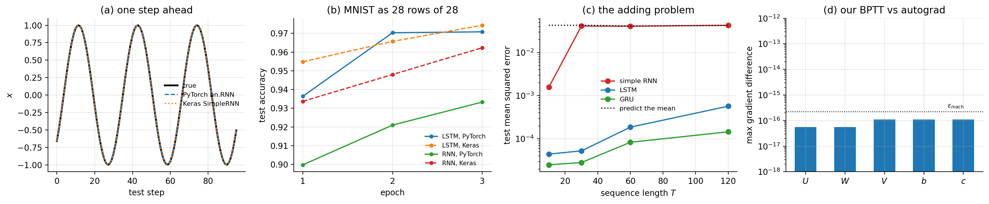
Figure 11.5: (a) One-step-ahead forecasts of the sine wave of Section Forecasting a sine wave on the held-out segment, from nn.RNN and from SimpleRNN; both lie on the true curve at a root-mean-square error of \(0.003\). (b) Test accuracy against epoch for MNIST read row by row, Table 11.1. (c) The adding problem: mean squared error against sequence length for the three cells, with the error of predicting the mean shown dotted. The simple RNN leaves the dotted line only at \(T=10\). (d) The largest disagreement between our BPTT recursion, Eqs. (11.15)–(11.18), and the same gradients from automatic differentiation, against the double-precision unit roundoff.
11.9. Summary and the programs#
A recurrent network is the architecture obtained by insisting that a model respect the ordering of its data and reuse its parameters along the time axis. The state-space form (11.3) makes it a learned dynamical system, and Section Where the recurrence comes from: a differential equation showed that the recurrence is not arbitrary but exactly the structure of an explicit time-stepping scheme for a differential equation.
Backpropagation through time is ordinary backpropagation on the unrolled graph, with the gradients from all steps summed into shared parameters. The forward pass is non-linear and bounded; the backward pass is linear and unbounded, and that asymmetry is the source of every difficulty in this chapter.
Theorem 11.1 makes the difficulty precise: the gradient across a lag is a product of Jacobians, bounded by \((\gamma\sigma_{\max}(\bm{W}))^{T-t}\), so it vanishes or explodes exponentially unless the network sits at the boundary. Measured on a network with \(\rho(\bm{W})=0.5\) over fifty-nine steps, the influence of the first state on the last fell by eighteen orders of magnitude. Clipping, Eq. (11.23), handles explosion cheaply and does nothing at all for vanishing.
The LSTM handles vanishing by giving the gradient an additive path, Eq. (11.27), whose Jacobian is a product of forget gates alone. The measurement in Section Why it works, and by how much should be kept in mind alongside the argument: at \(\bm{b}_f=0\) the LSTM transmits \(3.9\times10^{-18}\) over fifty-nine steps, no better than the vanilla RNN’s \(1.7\times10^{-18}\), and it is biasing the gate open that buys the ten to fifteen orders of magnitude. The architecture supplies the path; the initialisation decides whether training starts near it.
The experiment of Section The damped oscillator is the positive result. Trained on one trajectory of a damped oscillator and tested on a different initial condition, and then on a driven oscillator it had never seen, the network’s error was unchanged at three parts in ten thousand of the variance. It learned the update rule rather than the trajectory.
Three quantitative additions sharpen the picture. Corollary 11.2 converts Theorem 11.1 into a memory horizon \(\tau\), and fitting it to the measured decay gives \(\tau=1.45\) steps at \(\rho(\bm{W})=0.5\) and \(9.66\) at \(\rho=0.9\) – the usable range is narrow and it sits just below one. Proposition 11.3 shows that clipping is the projection onto a ball, hence a trust region that preserves the descent direction, which is why it can be applied unconditionally. And Proposition 11.4 gives the cell Jacobian exactly; measuring it against Eq. (11.29) shows the constant-error carousel to be a lower bound that understates the true gradient by one to five orders of magnitude, since the gate paths conduct as well.
Section The same networks in PyTorch and TensorFlow then checked all of it against the libraries. Our forward pass and our BPTT recursion agree with PyTorch and TensorFlow to \(4.4\times10^{-16}\), and asking autograd directly for \(\partial\bm{h}^{(T)}/\partial\bm{h}^{(1)}\) reproduces the product of Eq. (11.19) to a ratio of \(1.0000\): the vanishing gradient is a property of the composition, not of an implementation. The chapter closes with the experiment the theory demands. On the adding problem a simple recurrent network solves \(T=10\) and fails completely from \(T=30\) onwards, sitting exactly on the predict-the-mean baseline, while the LSTM and the GRU solve every length up to \(T=120\) at errors two to three orders of magnitude lower. That gap, at that lag, is Corollary 11.2 made visible.
The programs are in the directory
doc/BookML/BookPrograms/chapter11_recurrent_networks.
Every listing above appears there as a numbered file, and three modules run start to finish and reproduce the numbers quoted in the text:
rnn.py– the forward pass, BPTT, clipping, Adam and the LSTM cell of Eqs. (11.25)–(11.28).verify_rnn.py– the gradient check against central differences, the Jacobian-product measurements of Section Measuring it, and the forget-bias study of Section Why it works, and by how much.oscillator.py– the Runge-Kutta integrator, the training data and the generalisation experiment of Section The damped oscillator.cross_check_rnn.py– the three-way comparison of Section Do the three implementations agree?, the autograd measurement of Theorem 11.1, the exact cell Jacobian of Proposition 11.4 against Eq. (11.29), and the fitted memory horizon of Corollary 11.2.rnn_torch.py– the sine forecast, the row-by-row MNIST classification and the adding problem of Section The experiment the theory demands.rnn_tf.py– the first two of those in TensorFlow.mnist_data.py– a loader that reads MNIST from a local.npz, so that the programs run without network access.
The two measurement figures are generated by the script
doc/BookML/BookFigures/ch11_figures.py
and contain no hand-placed numbers. The two
schematics, Figures 11.1 and 11.4, are TikZ
drawings in the chapter source rather than plots; they carry no data and are
adapted from the course diagrams in rnnsetup.tex and
lstm.tex. The script render_tikz.py in the same directory
compiles them standalone to PNG, so that the notebook version of the chapter,
which cannot typeset TikZ, can display them.
11.10. Exercises#
11.10.1. Warm-up exercises#
Parameter counting. (a) How many parameters has a simple RNN with \(n_x=10\), \(n_h=64\), \(n_y=1\)? (b) How many has the LSTM of Eqs. (11.25)–(11.28) with the same dimensions, and the GRU of Eq. (11.32)? (c) How many would a feed-forward network need if the sequence of length \(T=200\) were flattened into one vector, and what happens when \(T\) changes?
The unrolled graph. Draw the computational graph of Eq. (11.4) for \(T=4\), marking every place \(\bm{W}\) appears. Use it to explain why \(\nabla_{\bm{W}}\mathcal{L}\) is a sum of four terms and not one.
Fixed points. For the autonomous map (11.6) with \(n_h=1\), \(\sigma_h=\tanh\) and \(b=0\), show that \(h^\star=0\) is always a fixed point, that it is stable for \(|W|<1\), and that a pitchfork bifurcation occurs at \(W=1\) producing two stable non-zero fixed points. Relate this to Theorem 11.1.
The bound. (a) Prove that \(\rho(\bm{A})\le\|\bm{A}\|_2\) for any square \(\bm{A}\), with equality when \(\bm{A}\) is normal. (b) Construct a \(2\times2\) matrix with \(\rho=0.5\) and \(\sigma_{\max}>2\), and explain what this implies about transient growth of the gradient. (c) Why does Theorem 11.1 use \(\sigma_{\max}\) rather than \(\rho\)?
Activations. Show that the logistic function has \(\gamma=\max|\sigma'|=1/4\) while \(\tanh\) has \(\gamma=1\). Deduce that a logistic recurrent network loses at least two bits of gradient per step regardless of its weights, and explain why \(\tanh\) is the standard choice.
The constant error carousel. Derive Eq. (11.29) from Eq. (11.27), stating clearly which term you are dropping and when that is justified. Then show that the diagonal part of Eq. (11.30) has norm at most one, so that the cell path alone can never cause explosion, and explain why Proposition 11.4 nevertheless leaves room for it.
The memory horizon. (a) Derive Corollary 11.2 and compute \(\tau\) for \(\gamma=1\) and \(\sigma_{\max}=0.9\), \(0.99\), \(0.999\). (b) How large must \(\sigma_{\max}\) be for a horizon of \(100\) steps, and what does Theorem 11.1 then say about the exploding regime? (c) Reproduce the fitted horizons quoted in Section Measuring it and explain why the fitted \(\tau\) is smaller than the one Eq. (11.21) predicts from \(\sigma_{\max}\).
Truncated backpropagation. (a) Derive the bound (11.22), stating what \(C\) collects. (b) For \(\tau=5\), find the truncation length \(k\) that keeps the bias below one per cent of the surviving gradient. (c) Implement truncated BPTT in
rnn.pyand confirm the bound numerically by comparing against the untruncated gradient.Clipping. (a) Prove Proposition 11.3. (b) Show that clipping each parameter array separately, rather than the concatenated gradient, does not in general preserve the direction, and construct a two-array example where the angle changes. (c) What happens to Adam’s second-moment estimate when clipping is active often, and does that argue for clipping before or after the optimiser state is updated?
The exact cell Jacobian. (a) Derive Proposition 11.4, being careful about which quantities \(\bm{o}^{(t-1)}\) depends on. (b) Bound \(\|\bm{R}^{(t)}\|_2\) in terms of the gate weight norms and \(\|\bm{c}^{(t-1)}\|_\infty\). (c) Explain, from Eq. (11.31), why the measured ratio in Section Why it works, and by how much gets worse rather than better when the input is scaled down.
The adding problem. Reproduce Section The experiment the theory demands and extend it. (a) At which \(T\) does the simple RNN fail, and how does that compare with the horizon \(\tau\) of its initialisation? (b) Set the forget-gate bias of the LSTM to zero and repeat. Does the LSTM still solve \(T=120\)? (c) Replace the LSTM by a simple RNN with \(\bm{W}\) initialised to the identity and ReLU activations – the identity RNN – and report where it sits between the two.
11.10.2. Project-style exercise: recurrent networks from scratch#
Part a: the machinery. Implement the forward pass (11.4) and backpropagation through time (11.15)–(11.18) in NumPy. Verify every entry of every gradient against central differences for at least three sequence lengths, and report the largest relative error.
Part b: the dynamics. Study the autonomous map (11.6) numerically for \(n_h=2\) and \(n_h=3\). Find fixed points, classify them by the eigenvalues of Eq. (11.7), and exhibit a limit cycle. Can you find chaotic behaviour, and how would you establish that it is chaotic rather than merely long-period?
Part c: measuring the theorem. Reproduce Section Measuring it: form the Jacobian product (11.19) explicitly and measure its norm against the lag for several spectral radii. Confirm the bound (11.20), report how loose it is, and explain the looseness. Then repeat with saturating inputs and describe what changes.
Part d: the oscillator. Reproduce Section The damped oscillator. Then push it: train on the undamped case \(\eta=0\) and test on \(\eta=0.2\), and vice versa. Train on one forcing frequency and test on another. Where does the learned update rule stop generalising, and does that boundary make physical sense?
Part e: clipping. Train with and without Eq. (11.23) over a range of thresholds \(\theta\) and sequence lengths. Record the distribution of gradient norms. At what sequence length does training fail without clipping, and does clipping ever hurt?
Part f: gates. Implement the LSTM of Eqs. (11.25)–(11.28) and the GRU of Eq. (11.32) from scratch, with verified gradients. Reproduce the forget-bias measurement of Section Why it works, and by how much for both. Then design a task that genuinely requires long memory – for instance, output the first element of the sequence at the final step, with \(T\) ranging from \(10\) to \(200\) – and plot the accuracy of the RNN, the LSTM and the GRU against \(T\) at matched parameter counts. This is the experiment that decides whether the gates are worth their cost.
Part g: against a library. Rebuild the same architectures in PyTorch or TensorFlow and verify that they agree with yours numerically: feed both the same weights and the same input and compare the forward and backward passes to machine precision. Check the library’s forget-gate bias initialisation, and measure what setting it to one does to your long-memory task from part f.