
8. Chapter 8: Neural Networks#
Chapter 5 closed with a remark that was left deliberately unexplained: logistic regression is a neural network with no hidden layer. Its linear predictor \(\bm{x}^{T}\bm{\theta}\) is a single artificial neuron, its sigmoid is that neuron’s activation function, and its cross entropy is the loss used to train classification networks throughout deep learning. This chapter makes good on the remark by inserting layers between the input and the output, so that the features fed to the final sigmoid are themselves learned rather than given.
That single change buys a great deal and costs a great deal. What it buys is universality: a network with one hidden layer can approximate any continuous function to arbitrary accuracy, which none of the linear models of the previous chapters can do. What it costs is every guarantee we have relied on. The cost function is no longer convex, so Section Convexity no longer applies and we can no longer say that the minimum we find is the minimum that exists. There is no closed form, no analogue of the normal equations, and no Karush-Kuhn-Tucker conditions to check the answer against. We are left with gradient descent and the chain rule.
Fortunately the chain rule is enough. The central result of this chapter, backpropagation, is nothing more than Eq. (1.51) applied systematically to a composition of layers, arranged so that the gradient with respect to all the parameters is obtained for the price of about two forward passes. It is the reverse-mode automatic differentiation of Section Automatic differentiation, specialised to the layered structure of a network and written out by hand.
8.1. Artificial neurons#
An artificial neuron takes several inputs, forms a weighted sum, adds a bias and passes the result through a non-linear function. Writing the inputs as \(x_i\), the weights as \(w_i\) and the bias as \(b\),
where \(f\) is the activation function and \(z\) the activation or pre-activation. The bias is needed for the same reason the intercept was needed in Section Scaling, centring and the intercept: without it the neuron is constrained to pass through the origin. Figure 8.1 is Eq. (8.1) drawn: the weighted sum on the left, the bias entering as an input of its own, and the non-linearity on the right.
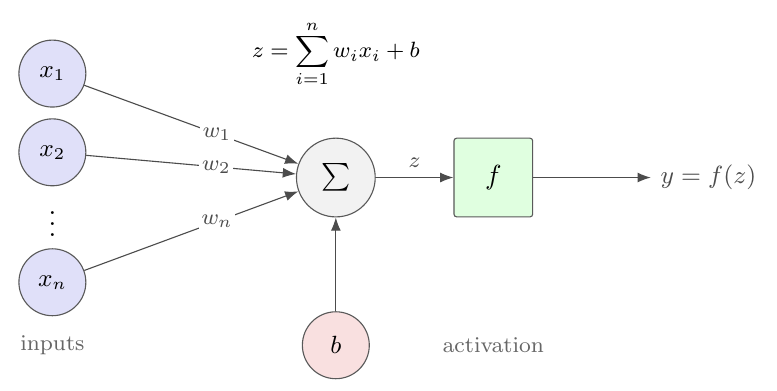
Figure 8.1: The artificial neuron of Eq. (8.1). The inputs \(x_i\) are combined linearly with the weights \(w_i\), the bias \(b\) is added – it is drawn as a separate input because that is what it is, an input permanently fixed at one – and the resulting pre-activation \(z\) is passed through the non-linear activation function \(f\) to give the output \(y\). Taking \(f\) to be the identity gives linear regression, the logistic function gives logistic regression, and the step function gives Rosenblatt’s perceptron.
Equation (8.1) is not new. Taking \(f\) to be the identity gives the linear model of Chapter 3; taking \(f=\sigma\), the logistic function of Eq. (5.3), gives logistic regression exactly; taking \(f\) to be the step function gives the perceptron, historically the first machine learning model, mentioned in Section Classification problems as the hard classifier that the soft one improved upon. A neuron is a familiar object under a new name.
In a network of such neurons the inputs \(x_i\) to one neuron are the outputs of the neurons in the preceding layer. A network is fully connected when each neuron receives a weighted sum of the outputs of all neurons in the previous layer, and feed-forward when the connections carry information in one direction only, from input to output, with no cycles.
8.2. Why one layer is not enough: the XOR problem#
The clearest motivation for hidden layers is a problem that a single neuron provably cannot solve. Consider the classical logic gates, with two binary inputs \(x_1,x_2\) and a binary target:
\(x_1\) |
\(x_2\) |
AND |
OR |
XOR |
|---|---|---|---|---|
0 |
0 |
0 |
0 |
0 |
0 |
1 |
0 |
1 |
1 |
1 |
0 |
0 |
1 |
1 |
1 |
1 |
1 |
1 |
0 |
Table 8.1: The AND, OR and XOR gates. The first two are linearly separable in the plane; the third is not.
Let us first try linear regression, using the design matrix of Eq. (1.1) with a column of ones for the intercept.
import numpy as np

X = np.array([[1, 0, 0], [1, 0, 1], [1, 1, 0], [1, 1, 1]], dtype=np.float64)
Xinv = np.linalg.pinv(X.T @ X)

for name, y in [("XOR", [0, 1, 1, 0]), ("OR", [0, 1, 1, 1]), ("AND", [0, 0, 0, 1])]:
    y = np.array(y, dtype=np.float64)
    theta = Xinv @ X.T @ y                     # Eq. (3.olssolution)
    print(f"{name}: theta = {np.round(theta, 3)}, "
          f"prediction = {np.round(X @ theta, 3)}")
The output is
XOR: theta = [ 0.5 -0.  -0. ], prediction = [0.5 0.5 0.5 0.5]
OR:  theta = [0.25 0.5  0.5 ], prediction = [0.25 0.75 0.75 1.25]
AND: theta = [-0.25 0.5  0.5 ], prediction = [-0.25 0.25 0.25 0.75]
Look at the first line. For the XOR gate the fitted slopes are exactly zero and the model predicts \(0.5\) for every input: the least-squares fit has found that the best linear function of \(x_1\) and \(x_2\) is the constant one. This is not a numerical accident. For XOR the two classes sit at opposite corners of the unit square, and any straight line separating \(\{(0,1),(1,0)\}\) from \(\{(0,0),(1,1)\}\) would have to pass on both sides of the square at once. The OR and AND gates, by contrast, are linearly separable, and the fitted values do at least order the outputs correctly.
Replacing the linear model by logistic regression does not help, since it changes the link function but not the linearity of the boundary:
from sklearn.linear_model import LogisticRegression

for name, y in [("XOR", [0, 1, 1, 0]), ("OR", [0, 1, 1, 1]), ("AND", [0, 0, 0, 1])]:
    y = np.array(y)
    logreg = LogisticRegression().fit(X, y)
    print(f"{name}: accuracy {logreg.score(X, y):.2f}")
XOR: accuracy 0.50
OR:  accuracy 0.75
AND: accuracy 0.75
Fifty per cent on XOR is exactly chance. The verdict is unambiguous and it is the historical one: a single layer of neurons, however trained, computes a linear decision boundary and there are elementary problems that no linear boundary solves. This observation stalled the field for the better part of two decades.
Figure 8.2 shows why, and the picture is more convincing than any amount of algebra. For AND and for OR a single straight line separates the classes, and a single neuron computes exactly such a line. For XOR the two classes occupy opposite corners of the square, and no line can be drawn with both filled squares on one side and both circles on the other. The failure is geometric, and it is complete: it is not that training was insufficient or the learning rate poorly chosen, but that the model class does not contain a solution.
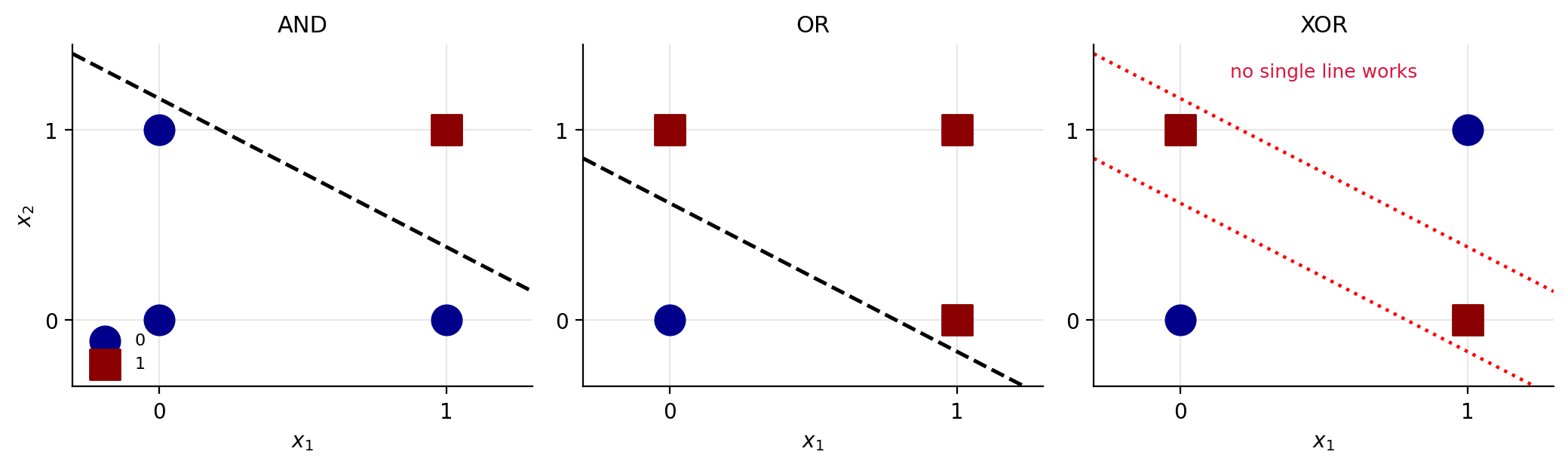
Figure 8.2: The three gates of Table 8.1 in the plane. AND and OR are linearly separable and a single neuron suffices; XOR is not, and no straight line separates the two classes.
The remedy is a hidden layer. With two hidden units the network can form two intermediate features – in effect, something like “\(x_1\) or \(x_2\)” and “not both” – and the output neuron combines them linearly. Using the implementation we develop in Section A neural network from scratch, a network with two inputs, two hidden nodes and two outputs learns all three gates perfectly:
X = np.array([[0, 0], [0, 1], [1, 0], [1, 1]], dtype=float)

for name, y in [("XOR", [0, 1, 1, 0]), ("OR", [0, 1, 1, 1]), ("AND", [0, 0, 0, 1])]:
    y = np.array(y)
    net = NeuralNetwork([2, 2, 2], "sigmoid", "classification",
                        gamma=1.0, epochs=4000, batch_size=4,
                        rng=np.random.default_rng(7)).fit(X, y)
    print(f"{name}: accuracy {np.mean(net.predict(X) == y):.2f}, "
          f"predictions {net.predict(X)}")
XOR: accuracy 1.00, predictions [0 1 1 0]
OR:  accuracy 1.00, predictions [0 1 1 1]
AND: accuracy 1.00, predictions [0 0 0 1]
Two hidden units and a non-linearity are the whole of the difference between \(0.50\) and \(1.00\).
Machine learning connection
It is worth being precise about what the hidden layer supplies, because it is easy to say “non-linearity” and stop there. A network with a hidden layer but linear activations computes \(\bm{W}^{2}(\bm{W}^{1}\bm{x}+\bm{b}^{1})+\bm{b}^{2}\), which is again an affine function of \(\bm{x}\) – the product of two matrices is a matrix, and no depth of linear layers escapes linearity. It is the composition of the linear map with a non-linear \(f\) that creates new features, and it is the reason every activation function in Section Activation functions is non-linear. Seen from Chapter 3, a network performs the basis expansion (3.4) with basis functions that are themselves fitted rather than chosen in advance.
8.3. Multilayer perceptrons and other architectures#
A fully connected feed-forward network with an input layer, one or more hidden layers and an output layer, whose neurons carry non-linear activation functions, is called a multilayer perceptron (MLP). This is the architecture we shall analyse in detail, and it is the one for which backpropagation takes its simplest form.
Several other architectures appear later in this book, and it is useful to know
what distinguishes them.
Convolutional networks replace full
connectivity by a small kernel slid across the input, so that each unit sees
only a local patch and the weights are shared across positions; this encodes
translation invariance and drastically reduces the parameter count, which is
why they dominate image processing. Recurrent networks feed the output
of a layer back into itself at the next time step, giving the network a memory
and making it suitable for sequences; the exploding-gradient problem of
Section Vanishing and exploding gradients is particularly acute there. Autoencoders
place a narrow bottleneck between an encoder and a decoder and are trained to
reproduce their own input, which forces the bottleneck to learn a compressed
representation – the non-linear counterpart of the principal component
analysis of Section Principal component analysis.
8.4. The universal approximation theorem#
Why should we expect a multilayer perceptron to be able to represent anything useful? The answer is a theorem, or rather a family of theorems refined over some thirty years, and it is worth stating carefully because the loose version in circulation claims both too much and too little.
Cybenko’s theorem.
The first result is due to Cybenko in 1989 [cybenko1989]. Let \(\sigma\) be any continuous sigmoidal function, meaning one with the limits
and let \(F(\bm{x})\) be a continuous function on the unit cube in \(d\) dimensions, \(\bm{x}\in[0,1]^{d}\). Then for every \(\epsilon>0\) there exists a network with a single hidden layer, \(f(\bm{x};\bm{\Theta})\) with \(\bm{\Theta}=(\bm{W},\bm{b})\), such that
In words: any continuous function on the unit cube in \(d\) dimensions can be approximated by a one-layer sigmoidal network to arbitrary accuracy.
A familiar shape of argument. Readers who have met the Stone-Weierstrass theorem for polynomial approximation, or the convergence criteria for Fourier series, will recognise the structure: a family of simple functions is shown to be dense in the space of continuous functions on a compact set. Cybenko’s proof proceeds by functional analysis, showing that if the closure of the span of the network functions were not everything, a non-zero signed measure would annihilate it, and then deriving a contradiction from the sigmoidal property. The result is an existence statement of exactly the kind Stone-Weierstrass provides for polynomials, and it should be regarded with the same mixture of reassurance and scepticism.
Hornik’s extension.
Hornik [hornik1991] generalised the result in two directions. First, the activation need only be non-constant and bounded, not specifically sigmoidal. Second, and more useful in a statistical setting, the approximation can be stated in mean square rather than uniformly. If the inputs are distributed with density \(p(\bm{x})\) on a domain \(D\) and the target has finite second moment,
then for every \(\epsilon>0\) there is a network with
Equation (8.5) is the statement one actually wants, because it is the expected squared error of Section The bias-variance tradeoff rather than a worst case over a cube the data may never visit. Hornik’s second point was that universality is a property of the two-layer architecture and not of any special feature of sigmoids.
What the condition really is. The conditions usually quoted – non-constant, bounded, monotonically increasing and continuous – are sufficient but not necessary. They were convenient for the original proofs, which leaned on the boundedness. The
sharp characterisation is due to Leshno, Lin, Pinkus and Schocken [leshno1993]: a feed-forward network with one hidden layer is a universal approximator if and only if the activation function is not a polynomial on any interval.
This is a much better statement, and it explains a good deal. It tells us at once that ReLU qualifies, although it is unbounded and so fails Cybenko’s hypothesis; that every function in Section Activation functions qualifies; and that the one activation which does not work is the linear one, which is a polynomial of degree one – recovering, from the general theory, the elementary observation of the notebox in Section Why one layer is not enough: the XOR problem that a network of linear layers collapses to a single linear map.
Which functions can be approximated. The theorems concern continuous functions on a compact domain. A discontinuous \(F\) cannot in general be approximated uniformly – near a jump, any continuous approximant must be wrong somewhere – although in the mean square sense of Eq. (8.5) a network may still do perfectly well, failing only on a set of small measure. Compactness matters too: nothing is claimed about behaviour outside the region where the approximation was constructed, which is the formal counterpart of the practical warning in Section Limitations, and a top-down view that networks extrapolate unpredictably.
What the theorems do not say. Three qualifications are essential, and all three are routinely forgotten.
First, the conditions apply to the hidden layer only. The output nodes are taken to be linear, so as not to restrict the range of the output values; a sigmoid output could never represent a function taking the value \(7\).
Second, and most importantly, none of the proofs gives any relation between the approximation error \(\epsilon\) and the number of hidden nodes, nor any bound on the magnitudes of \(\bm{W}\) and \(\bm{b}\). The required width may grow exponentially with the input dimension. This gap can be closed, and Section How wide? A constructive bound closes it for the rectifier in one dimension with an explicit construction and an explicit width. Worse, the theorems are pure existence results: they assert that suitable weights exist and say nothing whatever about whether gradient descent, on a non-convex cost, will find them. A guarantee of representability is not a guarantee of learnability, and the distance between the two is where the practical difficulty of deep learning lives.
Third, universality is not by itself remarkable. Polynomials are universal on a compact interval by Stone-Weierstrass, and so are Fourier series, splines and radial basis functions; none of these is regarded as a breakthrough. What distinguishes networks is not that they approximate but how economically they do so in high dimensions, and in particular that adding depth rather than width is empirically far more efficient. There are functions representable by a deep network with a number of units polynomial in the depth which provably require exponentially many units in a shallow one. The classical theorem, which concerns a single hidden layer, says nothing about this – so the result that justifies the field’s name is precisely the one the theorem does not cover. Section Why depth? An exact separation gives a case where the separation can be proved in half a page.
Machine learning connection
A useful way to hold the theorem in mind is to compare it with what we know about polynomials from Chapter 3. Polynomials are universal too, yet Figure 3.7 showed a degree-fourteen polynomial fit failing catastrophically – not because the function was unrepresentable but because the coefficients could not be estimated from a hundred noisy points. Universality is a statement about the model class; generalisation is a statement about the model class, the data and the estimator together, and it is governed by Eq. (2.52) rather than by any approximation theorem. A network large enough to approximate anything is also large enough to overfit anything, which is why Section Regularisation and hyperparameters exists.
8.4.1. How wide? A constructive bound#
The second qualification above – that no proof relates \(\epsilon\) to the number of hidden nodes – is a statement about those proofs, not about the problem itself. For a rectified activation in one dimension the question can be settled completely by an explicit construction, and it is worth doing, because the construction is three lines long and answers exactly the question the classical theorems evade.
The key observation is that a rectified network with one hidden layer is not merely dense in the continuous functions: it is the set of continuous piecewise linear functions, and the number of pieces can be read off the width.
Lemma 8.1 (Rectified networks are piecewise linear)
Let
be a network with one hidden layer of \(N\) rectified units and a linear output. Then \(g\) is continuous and piecewise linear with at most \(N+1\) affine pieces, and every breakpoint lies in the set \(\{-b_i/w_i : w_i\neq0\}\).
Proof
A unit with \(w_i=0\) is constant and contributes no breakpoint. A unit with \(w_i\neq0\) is affine on \((-\infty,-b_i/w_i]\) and affine on \([-b_i/w_i,\infty)\), so the only point at which it fails to be affine is \(t_i=-b_i/w_i\). The at most \(N\) points \(t_i\) cut the line into at most \(N+1\) open intervals, and on each of them every summand of Eq. (8.6) is affine; a finite sum of affine functions is affine. Continuity is inherited from the continuity of the rectifier. \qed
The converse is equally elementary – any continuous piecewise linear function with \(N\) breakpoints can be written in the form (8.6) – and it is what makes the following bound constructive rather than existential.
Theorem 8.2 (A width for every accuracy)
Let \(F\) be \(L\)-Lipschitz on \([a,b]\), that is \(|F(x)-F(x')|\le L|x-x'|\) for all \(x,x'\in[a,b]\). For every \(N\ge1\) there is a network (8.6) with \(N\) hidden rectified units such that
The hidden weights may all be taken equal to one and the hidden biases to \(-t_k\) with \(t_k=a+k(b-a)/N\); only the \(N+1\) output parameters depend on \(F\).
Proof
Write \(h=(b-a)/N\), \(t_k=a+kh\) for \(k=0,\dots,N\) and \(y_k=F(t_k)\), and let \(s_k=(y_{k+1}-y_k)/h\) be the slope of the chord over \([t_k,t_{k+1}]\), with the convention \(s_{-1}=0\). Define
For \(x\in[t_m,t_{m+1}]\) every rectifier with \(k\le m\) is active and every rectifier with \(k>m\) is not, so on that interval \(g\) is affine with slope \(\sum_{k=0}^{m}(s_k-s_{k-1})=s_m\), the sum telescoping. Since \(g(t_0)=y_0\) and the slope on \([t_k,t_{k+1}]\) is \(s_k\), induction gives \(g(t_k)=y_k\) for every \(k\): the network of Eq. (8.8) is exactly the piecewise linear interpolant of \(F\) at the \(N+1\) knots.
It remains to bound the interpolation error. Fix \(x\in[t_m,t_{m+1}]\) and write \(x=t_m+\theta h\) with \(\theta\in[0,1]\), so that \(g(x)=(1-\theta)y_m+\theta y_{m+1}\) and
The Lipschitz property gives \(|F(x)-F(t_m)|\le L\theta h\) and \(|F(x)-F(t_{m+1})|\le L(1-\theta)h\), whence
the last step because \(\theta(1-\theta)\le1/4\) on \([0,1]\). \qed
Equation (8.7) is the missing relation. Inverting it, accuracy \(\epsilon\) is reached with
hidden units – an explicit, finite and entirely unmysterious width. Nothing in the proof is an existence argument: Eq. (8.8) writes the weights down, and Fig. 8.4(a) plots the resulting network for \(N=4\) and \(N=16\).
The constant cannot be improved
Take \(F(x)=\mathrm{dist}(x,h\mathbb{Z})\), the triangular wave of period \(h\), which is \(1\)-Lipschitz. It vanishes at every knot \(t_k=kh\), so the interpolant of Eq. (8.8) is identically zero, while \(\sup|F|=h/2\). The bound (8.7) is therefore attained exactly, and the factor two in the denominator is the best possible for the class of \(L\)-Lipschitz functions.
Both statements can be checked numerically. The program \verb!universal.py! builds the network of Eq. (8.8) – it trains nothing – and measures its error on a grid of \(200\,001\) points:
=== 1. the explicit construction of Theorem 8.relurate ===
  target F(x) = sin(2 pi x) on [0,1], Lipschitz constant L = 2 pi
     N    sup error   bound L/2N   ratio
     2    1.000e+00    1.571e+00   0.6366
     8    7.038e-02    3.927e-01   0.1792
    32    4.792e-03    9.817e-02   0.0488
   128    3.011e-04    2.454e-02   0.0123
   512    1.882e-05    6.136e-03   0.0031
     N    sup error   bound L/2N   ratio
     2    2.500e-01    2.500e-01   1.0000
     8    6.250e-02    6.250e-02   1.0000
    32    1.562e-02    1.562e-02   1.0000
   128    3.905e-03    3.906e-03   0.9997
   512    9.763e-04    9.766e-04   0.9997
The second table is the worst case of the notebox: the ratio is one to every figure the grid can resolve, and the small shortfall at large \(N\) is the resolution of the grid, not a failure of the theory. The first table says something else worth noticing. For a smooth target the error falls like \(N^{-2}\), not like \(N^{-1}\): that is the classical estimate \(\|F-g\|_\infty\le h^{2}\|F''\|_\infty/8\) for piecewise linear interpolation, and it is the first sign that the Lipschitz class is a pessimistic yardstick. Sharper rates of this kind, for deep rectified networks and for targets with \(s\) derivatives, are the subject of [yarotsky2017]; the whole approximation-theoretic picture is surveyed in [pinkus1999].
8.4.2. The curse of dimensionality#
Theorem 8.2 is one-dimensional, and the dimension is where the difficulty lies. Repeating the construction on \([0,1]^{d}\) means covering the cube with a grid of side \(h\) and interpolating on it, which takes of the order of \(h^{-d}\) pieces; to reach accuracy \(\epsilon\) for an \(L\)-Lipschitz target one therefore needs of the order of
units. With \(L=1\) and \(\epsilon=10^{-1}\) this is five units in one dimension, about \(10^{3}\) in three, and about \(10^{12}\) in ten. The exponent is the input dimension, and no cleverness in the construction removes it.
Nor is this an artefact of the particular construction. The class of \(L\)-Lipschitz functions on \([0,1]^{d}\) contains, for every grid of side \(h\), a family of \(2^{h^{-d}}\) functions obtained by placing a bump of height \(Lh/2\) on each cell with an independent sign; any two of them differ by \(Lh/2\) somewhere, so distinguishing them requires at least \(h^{-d}\) bits and hence at least that many parameters. Made precise – the parameters must be chosen by a map depending continuously on the target – this is the theorem of DeVore, Howard and Micchelli [devore1989]: no approximation scheme with \(N\) parameters achieves error better than \(c_dLN^{-1/d}\) uniformly over the Lipschitz ball. A network with one hidden layer of width \(N\) has \(N(d+2)+1\) parameters, so it is covered by the theorem, and the exponent in Eq. (8.12) is sharp.
The way out is not a better architecture but a smaller class of targets. The classical result of this kind is Barron’s [barron1993].
Theorem 8.3 (Barron)
Let \(F:\mathbb{R}^{d}\rightarrow\mathbb{R}\) have a Fourier representation \(F(\bm{x})=\int e^{\imath\bm{\omega}\cdot\bm{x}}\hat{F}(\bm{\omega})\,d\bm{\omega}\) with finite first moment,
Then for every \(N\) and every probability measure \(\mu\) supported in the ball of radius \(r\) there is a network with one hidden layer of \(N\) sigmoidal units for which
The rate \(N^{-1}\) in the squared error contains no \(d\) at all. The mechanism deserves a sentence, because it explains where the dimension went. The Fourier representation exhibits \(F-F(\bm{0})\) as a member of the closed convex hull of a set \(\mathcal{G}\) of individual ridge functions of norm at most \(2rC_F\), so \(F\) is a limit of averages of elements of \(\mathcal{G}\); and if \(N\) elements are drawn independently from the mixing distribution, the mean squared error of their average is the variance of a single draw divided by \(N\), which is at most \((2rC_F)^{2}/N\). Some particular draw must be at least as good as the average, so a network of width \(N\) with that error exists. This averaging argument is due to Maurey. The dimension enters only through \(C_F\), and for the functions one actually wants to fit – superpositions of a moderate number of ridge directions, which is precisely what a network is – \(C_F\) does not grow with \(d\).
We can watch this happen. The target \(F(\bm{x})=M^{-1}\sum_m c_m\cos(\kappa\,\bm{a}_m\cdot\bm{x})\) with \(M=12\) unit ridge directions has a Fourier transform consisting of point masses at \(\pm\kappa\bm{a}_m\), so its Barron norm is known exactly, \(C_F=\kappa M^{-1}\sum_m|c_m|\), and it does not depend on \(d\); drawing \(\bm{x}\) uniformly from the unit ball fixes \(r=1\) in every dimension as well. Theorem 8.3 therefore predicts the same bound in \(d=1\), \(5\) and \(20\):
  kappa = 8:  C_F = 6.9124
      N       d = 1       d = 5      d = 20   bound (2 C_F)^2/N
      4   1.296e-02   2.689e-02   3.186e-02           4.778e+01
     16   2.330e-04   6.902e-03   2.202e-03           1.195e+01
     64   2.693e-04   1.247e-03   6.183e-04           2.986e+00
    128   1.850e-04   7.520e-04   6.779e-04           1.493e+00
  measured slopes of log(mse) against log(N):   -0.77  -1.08  -1.14   (Theorem 8.barron: -1)
  ratio of the d = 20 error to the d = 1 error at N = 128:  3.7
Three things are worth reading off. The bound holds, and with an enormous margin – it is a worst-case bound over the whole Barron class, and this particular target is far from the worst. The measured decay is close to the predicted \(N^{-1}\) in every dimension. And the error at \(d=20\) exceeds the error at \(d=1\) by a factor of under four, a constant, not by anything resembling the exponential of Eq. (8.12). It is the dimension in the exponent that the Barron class removes; a moderate constant remains. Set against Eq. (8.12), where reaching a fixed accuracy at \(d=20\) would take more units than there are atoms in the room, this is the whole difference between a usable method and an impossible one.
8.4.3. Why depth? An exact separation#
The third qualification – that the classical theorem concerns one hidden layer and so says nothing about depth – can also be repaired, and in one dimension the repair is completely elementary. We exhibit a function that a deep network of \(2k\) units represents exactly, and that no shallow network with fewer than \(2^{k}-1\) units can approximate at all.
Definition 8.4 (The tent map and the sawtooth)
Let
so that \(T(x)=2x\) on \([0,\tfrac12]\) and \(T(x)=2-2x\) on \([\tfrac12,1]\), and let \(s_k=T\circ T\circ\cdots\circ T\) be the \(k\)-fold composition.
Equation (8.15) is one hidden layer of two rectified units followed by a linear combination. Composing it \(k\) times is therefore a network with \(k\) hidden layers of two units each: \(2k\) units and \(6k\) parameters in all.
Lemma 8.5 (The sawtooth)
\(s_k\) maps \([0,1]\) onto \([0,1]\), is piecewise linear with exactly \(2^{k}\) affine pieces of slope \(\pm2^{k}\), and satisfies
Proof
Induction on \(k\). For \(k=1\) the statement is Eq. (8.15). Assume it for \(k\) and write \(s_{k+1}=s_k\circ T\). The map \(T\) carries \([0,\tfrac12]\) affinely onto \([0,1]\) and carries \([\tfrac12,1]\) affinely onto \([0,1]\) with the orientation reversed. Hence \(s_{k+1}\) restricted to \([0,\tfrac12]\) is a copy of \(s_k\) compressed by a factor two, and restricted to \([\tfrac12,1]\) is a reflected copy: \(2^{k}+2^{k}=2^{k+1}\) pieces in all, each of slope \(\pm2\cdot2^{k}\). The points \(j/2^{k+1}\) are the preimages of the points \(j/2^{k}\), and the alternation of the values is preserved by both branches. \qed
Theorem 8.6 (Depth against width)
Let \(g\) be a network with a single hidden layer of \(N\) rectified units, as in Eq. (8.6). If \(N\le2^{k}-2\) then
Proof
Suppose on the contrary that \(\|g-s_k\|_\infty<\tfrac12\), and put \(x_j=j/2^{k}\) for \(j=0,\dots,2^{k}\). By Eq. (8.16) we then have \(g(x_j)<\tfrac12\) for even \(j\) and \(g(x_j)>\tfrac12\) for odd \(j\), so the continuous function \(g-\tfrac12\) changes sign on each of the \(2^{k}\) intervals \((x_j,x_{j+1})\) and has a zero \(z_j\) in each. These zeros are distinct and ordered, \(z_0<z_1<\cdots<z_{2^{k}-1}\).
No two consecutive zeros can lie in the same affine piece of \(g\). For if \(z_j\) and \(z_{j+1}\) both lay in a piece \(P\), then \(g-\tfrac12\) would be affine on \(P\) with two distinct zeros and hence identically zero there; but \(x_{j+1}\in(z_j,z_{j+1})\subset P\), so \(g(x_{j+1})=\tfrac12\), contradicting the strict inequality above. The \(2^{k}\) zeros therefore lie in \(2^{k}\) distinct pieces, so \(g\) has at least \(2^{k}\) pieces, and Lemma 8.1 gives \(N+1\ge2^{k}\). This contradicts \(N\le2^{k}-2\). \qed
The separation is exponential and it is exact. A network of depth \(k\) with two units per layer – \(2k\) units, growing linearly in \(k\) – reproduces \(s_k\) with no error whatever, while any network with a single hidden layer needs at least \(2^{k}-1\) units, growing exponentially, merely to come within a half. At \(k=10\) the deep network has twenty units and the shallow one needs more than a thousand.
Both halves of the statement can be measured. Composing the tent map and counting the affine pieces of the result confirms Lemma 8.5:
     k   units in the deep net   linear pieces measured   2^k
     1                       2                        2      2
     4                       8                       16     16
     8                      16                      256    256
Fitting shallow networks of increasing width to \(s_3\), which has eight pieces and therefore requires \(N\ge7\), produces the wall the theorem predicts:
   k = 3, s_k has 8 pieces, the theorem needs N >= 7
      N   sup error   pieces of the fit   N+1
      2      0.5002                   2      3
      4      0.5212                   2      5
      8      0.5506                   6      9
     16      0.0096                  14     17
     32      0.0067                  25     33
     64      0.0031                  54     65
The number of pieces never exceeds the \(N+1\) of Lemma 8.1, and whenever it falls below eight the error sits at or above the \(1/2\) of Theorem 8.6 – including at \(N=8\), where the width is sufficient in principle but training produced a network with only six live pieces and the theorem then applies to that network. The whole picture is Fig. 8.3.
Theorem 8.6 is the simplest member of a family. Telgarsky proved a version separating networks of any fixed depth from networks of slightly smaller depth [telgarsky2016], and Mont’ufar and co-workers counted the linear regions of a general rectified network [montufar2014], finding a number that grows exponentially in the depth but only polynomially in the width. The mechanism is always the one in Lemma 8.5: composition multiplies the number of pieces, addition merely adds them. This is the result the name of the field refers to, and it is the one Cybenko’s statement cannot see.
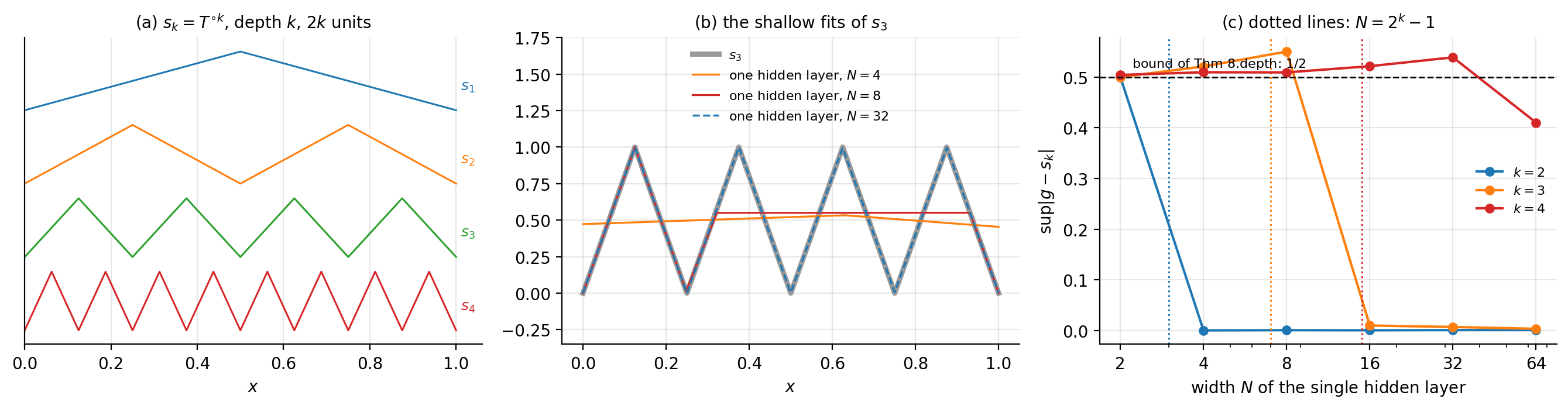
Figure 8.3: Depth against width. (a) The sawtooth \(s_k\) of Definition 8.4, computed exactly by a rectified network of depth \(k\) with two units per layer; the number of teeth doubles with each layer while the number of units grows by two. (b) Single-hidden-layer fits of \(s_3\): at \(N=4\) and \(N=8\) the network is flat at about \(1/2\), which is the best a function with too few pieces can do, and at \(N=32\) it reproduces \(s_3\) exactly. (c) The measured supremum error against the width, with the threshold \(N=2^{k}-1\) of Theorem 8.6 marked by the dotted vertical lines and the guaranteed error \(1/2\) by the horizontal one.
8.4.4. Representability is not learnability#
Every result so far is a statement about which functions a network contains. Training is a different question, and the gap between the two is not a technicality. The construction of Theorem 8.2 places the kinks at \(t_k=a+kh\) and computes the output weights directly from \(F\); gradient descent has to find both from a random start, on a cost function that Section Convexity tells us is not convex. Running the two side by side at identical widths, on the same target \(\sin2\pi x\):
     N   constructed   default init   kinks spread   ratio
     2     1.000e+00      1.000e+00      9.170e-01     0.9
     4     2.105e-01      1.108e+00      9.170e-01     4.4
     8     7.038e-02      1.837e-01      8.465e-02     1.2
    16     1.885e-02      7.203e-02      5.557e-02     2.9
    32     4.792e-03      4.279e-02      1.660e-02     3.5
    64     1.203e-03      4.386e-02      6.359e-03     5.3
Two things are visible. The first is that the default initialisation is a handicap in its own right: PyTorch draws \(w_i\) and \(b_i\) from \(\mathcal{U}(-1,1)\), so the kink \(-b_i/w_i\) falls inside the interval of interest for only a minority of the units, and the rest are dead from the start, contributing nothing and receiving no gradient. Spreading the kinks uniformly over \([0,1]\) – which is exactly where Eq. (8.8) puts them – improves matters at every width, and is a concrete instance of the general point of Section Weight initialisation.
The second is that even with the kinks well placed, training does not reach the constructed network, and the shortfall grows with the width: a factor \(1.2\) at \(N=8\) and \(5.3\) at \(N=64\). The exception at \(N=4\), where every seed lands in the same poor local minimum, is a reminder that these are non-convex problems and that the failure need not be monotone. The theorem guarantees that a set of weights exists; it says nothing about whether the trajectory of Adam passes anywhere near them. This is the honest reading of the universal approximation theorem. It removes representability as an excuse and leaves optimisation and generalisation as the two real problems, which are the subjects of Chapter 4 and of Section Regularisation and hyperparameters respectively. Figure 8.4 collects the three measurements.
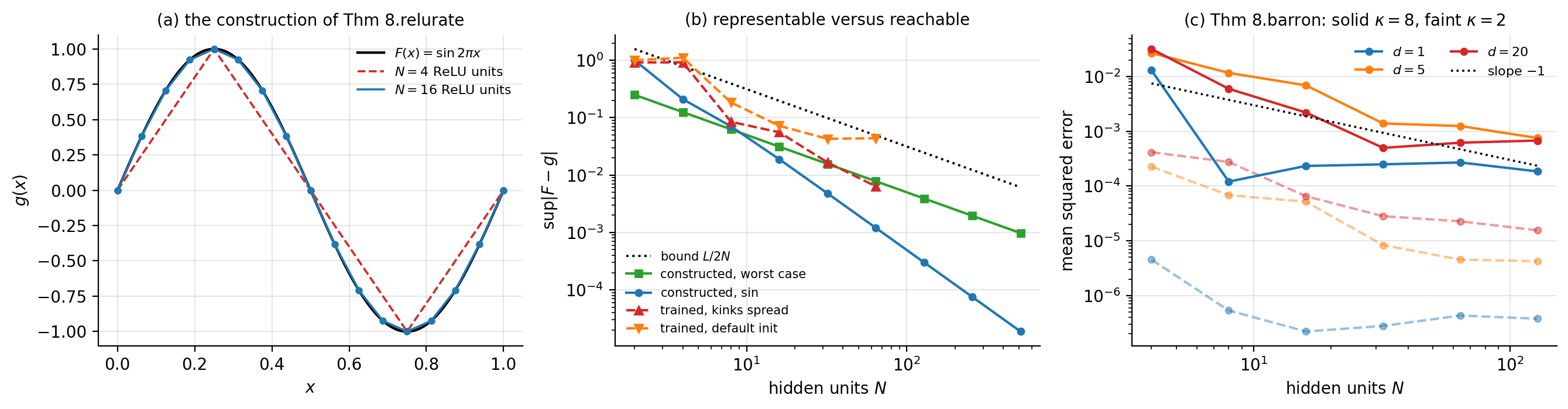
Figure 8.4: The quantitative content of Section The universal approximation theorem. (a) The network of Eq. (8.8), whose weights are written down rather than trained, for \(N=4\) and \(N=16\) hidden rectified units; the markers are the knots \(t_k\) at which it interpolates. (b) Supremum error against width: the bound (8.7), the constructed network for a smooth and for a worst-case Lipschitz target, and what Adam achieves at the same widths from two initialisations. The gap between the solid and the dashed curves is the distance between representability and learnability. (c) Barron’s rate (8.14) measured in \(d=1\), \(5\) and \(20\) for two values of the Barron norm; the slope is the predicted \(-1\) and it does not change with the dimension.
8.5. Notation and the feed-forward pass#
We now fix notation, and it repays care: almost every difficulty students have with backpropagation is a difficulty with indices rather than with calculus.
Layers are numbered \(l=0,1,\dots,L\), with \(l=0\) the input layer, \(l=L\) the output layer, and \(M_l\) the number of nodes in layer \(l\). The activation of node \(j\) in layer \(l\) is
where \(w_{ij}^{l}\) is the weight connecting node \(i\) of layer \(l-1\) to node \(j\) of layer \(l\), and \(b_j^{l}\) is the bias of node \(j\) in layer \(l\). The output of the node is obtained by applying the activation function,
with \(a_i^{0}=x_i\) the network inputs. In matrix-vector form, Eqs. (8.18) and (8.19) become
with \(f\) applied element-wise. Evaluating Eq. (8.20) for \(l=1,\dots,L\) is the feed-forward pass, and the network output is \(\tilde{\bm{y}}=\bm{a}^{L}\).
Figure 8.5 shows the whole object with these labels attached, and Figure 8.6 shows a single node of it, which is where the index convention has to be learned. The point to fix in mind is that the superscript on \(w_{ij}^{l}\) names the layer the weight arrives at, that the first subscript names the node it leaves and the second the node it arrives at, and that the sum in Eq. (8.18) is therefore over the first index. Every other convention in circulation is a permutation of this one, and the only thing that matters is to choose one and never deviate from it.
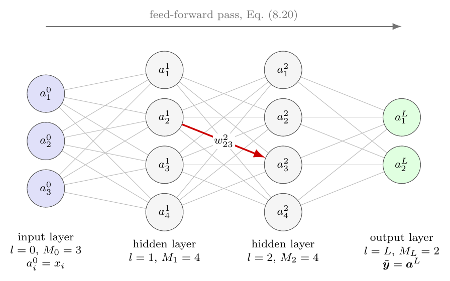
Figure 8.5: A fully connected feed-forward network in the notation of Section Notation and the feed-forward pass, here with \(L=3\). Layer \(l\) has \(M_l\) nodes and node \(j\) of that layer carries the output \(a_j^{l}\) of Eq. (8.19); the input layer holds \(a_i^{0}=x_i\) and the output layer the prediction \(\tilde{\bm{y}}=\bm{a}^{L}\). Every node of one layer is connected to every node of the next, and the highlighted edge carries the weight \(w_{23}^{2}\), from node \(i=2\) of layer \(l-1=1\) to node \(j=3\) of layer \(l=2\): the superscript names the receiving layer and the first index names the sending node.
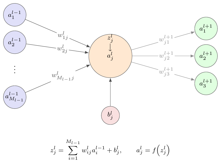
Figure 8.6: The index convention of Eqs. (8.18) and (8.19), seen from a single node. Node \(j\) of layer \(l\) collects the outputs \(a_i^{l-1}\) of all \(M_{l-1}\) nodes of the previous layer, weighted by \(w_{ij}^{l}\), adds its own bias \(b_j^{l}\) to form the pre-activation \(z_j^{l}\), and applies \(f\) to obtain \(a_j^{l}\), which it then sends on to every node of layer \(l+1\) through the weights \(w_{jk}^{l+1}\). The first index of a weight always refers to the layer below and the second to the layer above, so that the sum in Eq. (8.18) runs over the first index and the sum in the backpropagation equation (8.64) runs over the second.
The cost of one forward pass is dominated by the matrix products: layer \(l\) requires \(M_{l-1}M_l\) multiplications, so the whole pass costs \(\bigO\!\left(\sum_l M_{l-1}M_l\right)\), which is also the number of weights. This is why the operations of Chapter 1 matter here: a network is, computationally, a sequence of level-3 BLAS calls interleaved with element-wise non-linearities, and Section Arrays in practice: numpy, BLAS and LAPACK explains why one must let the library perform them.
Batches.
In practice one propagates a whole minibatch at once. Stacking \(n\) samples as rows of \(\bm{A}^{l-1}\in\mathbb{R}^{n\times M_{l-1}}\), the forward pass reads
with the bias added by broadcasting. This is the form the code of Section A neural network from scratch uses, and note that it transposes the convention of Eq. (8.20): with samples in rows, \(\bm{W}^{l}\) appears untransposed. Both conventions are common and mixing them is the single most frequent source of shape errors.
8.6. Activation functions#
The activation function must be non-linear, by the argument of the notebox in Section Why one layer is not enough: the XOR problem and by the sharp characterisation of Section The universal approximation theorem, and for gradient-based training it must be differentiable almost everywhere. Beyond that the choice is open, and it matters more than one might expect: the history of deep learning is to a surprising extent the history of replacing one activation function by another.
The property to keep in view throughout is the derivative, because it is \(f'\) and not \(f\) that enters the backpropagation recursion (8.66) and therefore decides whether a gradient survives its passage through a layer.
8.6.1. Saturating activations#
The logistic or sigmoid function of Eq. (5.3),
was the standard choice for decades and is the one Cybenko’s theorem was proved for. Its derivative is expressible in the function value alone, which is convenient, and it never exceeds \(\tfrac14\) – which, as Section Vanishing and exploding gradients shows, is fatal in deep networks. Its output is also strictly positive with mean near \(\tfrac12\), so the inputs to the next layer are not centred, which slows learning further.
The hyperbolic tangent \(\tanh(z)=2\sigma(2z)-1\), with \(\tanh'(z)=1-\tanh^{2}(z)\), is a rescaled sigmoid mapping onto \((-1,1)\). Its output is centred on zero and its derivative reaches \(1\) rather than \(\tfrac14\); it is consistently the better of the two and there is no good reason to prefer the logistic function in a hidden layer. Both nevertheless saturate: for \(|z|\) large the derivative is essentially zero and the unit stops learning.
8.6.2. The rectified family#
The rectified linear unit,
broke the deadlock. It is trivial to compute, it does not saturate for positive arguments so the gradient passes through undiminished, and it produces genuinely sparse activations since about half the units output zero. Its derivative is undefined at the origin, which in practice is assigned the value zero and never noticed.
ReLU has one characteristic failure, the dying ReLU. If a unit’s weights are updated so that its input is negative for every training sample, it outputs zero always; its gradient is then zero as well, so it can never recover, and the unit is dead for the remainder of training. With a large learning rate a substantial fraction of a network can die this way – in bad cases half of it.
Three repairs give the negative branch a non-zero slope. The leaky ReLU uses a fixed small slope,
so the gradient never vanishes entirely. PReLU makes \(\alpha\) a parameter learned by backpropagation like any other, one per channel. The exponential linear unit
does the same more smoothly, saturating at \(-\alpha\) for large negative arguments so that the unit output has a mean nearer zero, at the cost of an exponential. SELU is ELU with two particular constants chosen so that, under conditions on the initialisation, the activations of successive layers converge to zero mean and unit variance automatically – self-normalising, and so an alternative to the batch normalisation of Section Regularisation and hyperparameters.
All of these are piecewise linear or piecewise smooth with a kink at the origin. The next family removes the kink.
8.6.3. Smooth gated activations: GELU and its relatives#
The Gaussian error linear unit takes a different view of what an activation is doing. Rather than thresholding the input, it weights the input by the probability that it is positive:
where \(\Phi\) is the cumulative distribution function of the standard normal distribution met in Eq. (2.3). A unit whose input is large and positive is passed through essentially unchanged, since \(\Phi\to1\); one whose input is large and negative is suppressed, since \(\Phi\to0\); and in between the suppression is graded rather than abrupt. ReLU is the limiting case in which \(\Phi\) is replaced by the step function, that is in which the gating is deterministic rather than probabilistic.
Because the error function is expensive, implementations use the approximation
which agrees with Eq. (8.26) to better than \(5\times10^{-4}\) everywhere on \([-8,8]\) and is what most frameworks compute by default.
Two close relatives replace the Gaussian gate by a cheaper one. Swish, also called SiLU, gates with the logistic function,
and Mish gates with a \(\tanh\) of the softplus,
The softplus \(\ln(1+e^{z})\) itself is a smooth approximation to ReLU and appears mainly where a strictly positive output is needed, as when a network predicts a variance.
What these functions have in common, and why it matters. All three are smooth, all three are non-monotone, and all three have a derivative exceeding one somewhere. These are not incidental.
The non-monotonicity is easily quantified. Each dips below zero for moderately negative arguments before returning: GELU attains its minimum \(-0.170\) at \(z=-0.752\), Swish \(-0.278\) at \(z=-1.279\), and Mish \(-0.309\) at \(z=-1.192\). A small negative response is therefore preserved rather than discarded, which is the intended contrast with ReLU, and the function is not a squashing function in the sense of any of the classical theorems – it remains a universal approximator because it is not a polynomial, by Section The universal approximation theorem, which is precisely the situation the sharper characterisation was needed for.
The derivative maxima are \(1.129\) for GELU, \(1.100\) for Swish and \(1.089\) for Mish, against \(1\) for \(\tanh\) and \(\tfrac14\) for the sigmoid. A factor slightly greater than one in Eq. (8.71) means these activations can mildly amplify a gradient rather than only attenuate it, which is a genuine advantage in depth; it also means they cannot be relied on to damp an exploding gradient, so the clipping of Section Regularisation and hyperparameters remains necessary.
The smoothness matters for a reason that has nothing to do with classification. ReLU has a discontinuous first derivative and no second derivative at the origin, so any method requiring curvature – and any application in which the network’s output is differentiated, as when solving differential equations – is compromised. This is why the GELU family is the default choice for physics-informed networks, a point we return to in the next chapter.
Gated linear units. A final family generalises the idea by learning the gate. A gated linear unit splits a layer’s output in two and uses one half to gate the other,
with \(\circ\) the Hadamard product. Replacing the logistic gate by GELU gives GeGLU and by Swish gives SwiGLU; the latter is used in most current large language models. Note that these are not activation functions in the sense of the rest of this section – they are layers, with their own parameters, and they double the number of weights for a given output width.
8.6.4. Which activation should we use?#
The empirical ordering, on which the literature is reasonably consistent, is that the GELU and ELU families perform better than leaky ReLU and its variants, which perform better than ReLU, which performs better than \(\tanh\), which performs better than the logistic function.
That ordering should be read with great caution, and it is worth measuring rather than repeating. Table 8.2 gives the test accuracy of a network with three hidden layers of thirty units on the digits data, averaged over five random seeds with the standard deviation across seeds.
Activation |
Test accuracy |
Final training loss |
|---|---|---|
sigmoid |
\(0.8900\pm0.0096\) |
\(0.2971\) |
\(\tanh\) |
\(\mathbf{0.9722\pm0.0039}\) |
\(0.0048\) |
ReLU |
\(0.9672\pm0.0083\) |
\(0.0009\) |
leaky ReLU |
\(0.9672\pm0.0071\) |
\(0.0009\) |
ELU |
\(0.9672\pm0.0044\) |
\(0.0011\) |
GELU |
\(0.9694\pm0.0061\) |
\(0.0010\) |
Swish |
\(0.9661\pm0.0054\) |
\(0.0010\) |
Mish |
\(0.9672\pm0.0048\) |
\(0.0010\) |
Table 8.2: Test accuracy of a \(64\)-\(30\)-\(30\)-\(30\)-\(10\) network on the digits data after \(60\) epochs, as mean and standard deviation over five random seeds. Only the sigmoid is clearly separated from the rest.
The table is worth more than the ordering it fails to confirm. One result is unambiguous: the sigmoid is far behind, by eight percentage points and many standard deviations, and its training loss is two orders of magnitude higher – with three hidden layers the attenuation of Section Vanishing and exploding gradients is already severe. That much of the received wisdom is solidly reproduced.
The rest of the table is a single cluster. The seven non-saturating activations span \(0.9661\) to \(0.9722\), a range of \(0.006\), while the standard deviation across seeds is between \(0.004\) and \(0.008\) – so the spread between the methods is smaller than the spread between random seeds of the same method. On this evidence the claimed ordering among them cannot be distinguished from noise, and \(\tanh\), which the ordering places second from last, is nominally the best. Note also that the training losses are nearly identical while the test accuracies differ, so what little variation there is comes from generalisation and not from optimisation.
The honest conclusion is that on a problem of this size the choice among the non-saturating activations does not matter much, and that a paper reporting a single run and declaring a winner among them would be reporting seed noise. The differences do become real at greater depth, in transformers, and where the smoothness itself is needed; they are not real here. This is also a reminder of Section The central limit theorem: with \(360\) test samples the standard error of an accuracy near \(0.97\) is about \(0.009\), so a difference of \(0.006\) was never going to be resolvable. Figure 8.7 shows the same data with error bars, which makes the point at a glance.
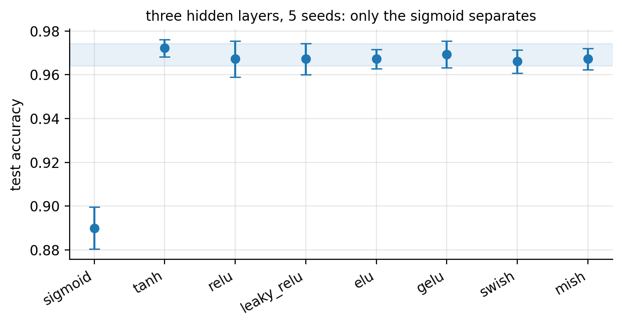
Figure 8.7: The data of Table 8.2 plotted with error bars of one standard deviation over five seeds. The shaded band spans the seven non-saturating activations; they are mutually indistinguishable, while the sigmoid lies far below.
Three further caveats apply to the literature ordering. It is confounded with architecture, since GELU rose to prominence together with transformers and is best attested there. Runtime matters: ReLU is a comparison and a multiplication, while GELU as computed by Eq. (8.27) requires a \(\tanh\) and a cubic, which on large models is not negligible. If runtime is a concern, leaky ReLU with the default \(\alpha=0.01\) avoids both the dying-unit problem and the cost, without introducing a hyperparameter worth tuning.
As a working rule: ReLU is a sound default and the right thing to try first; move to leaky ReLU or ELU if units are dying; use GELU or Swish in transformers, in very deep networks, and wherever the network output must be differentiated. Reserve \(\tanh\) for the cases where a bounded activation is genuinely wanted, and use the logistic function in a hidden layer only when reproducing an old result.
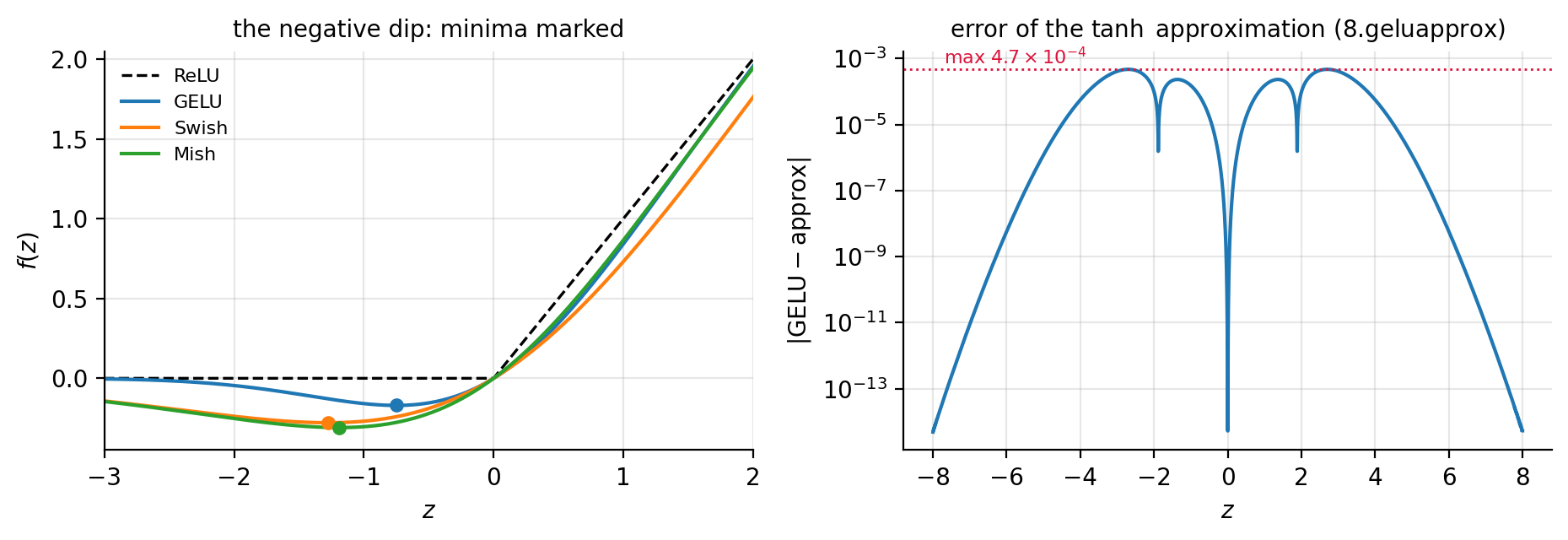
Figure 8.8: Left: GELU, Swish and Mish against ReLU, with the minimum of each marked – all three dip below zero and are therefore non-monotone. Right: the error of the \(\tanh\) approximation (8.27) to the exact GELU (8.26), which nowhere exceeds \(4.7\times10^{-4}\).
Figure 8.9 collects the three families with their derivatives. The bottom row is the one to study. The saturating functions have derivatives that vanish in both tails, and the sigmoid’s never exceeds \(\tfrac14\); the rectified functions have derivative exactly one on the positive axis and zero or nearly zero on the negative; the smooth gated functions have derivatives that rise slightly above one near the origin and decay smoothly on both sides. Reading the recursion (8.66) through these three panels explains the empirical ordering better than any list of benchmark numbers.
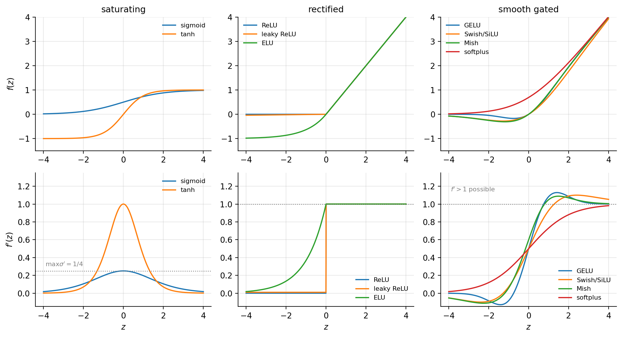
Figure 8.9: Nine activation functions in three families (top) and their derivatives (bottom). Only the derivative enters the backpropagation recursion (8.66). Dotted lines mark \(\max\sigma'=1/4\) in the left panel and \(f'=1\) in the other two.
The output layer is not a free choice. Everything above concerns hidden layers. The output activation is fixed by the range of the target, exactly as the loss is fixed by its distribution in Section Deriving least squares from a probability distribution: the identity for regression, the sigmoid for binary classification, the softmax of Eq. (5.27) for \(K\) classes, and softplus or an exponential where the output must be positive. Choosing these independently of the loss is one of the more common ways to produce a network that trains to something meaningless.
8.7. The cost function and the optimisation problem#
Collect all weights and biases into a single parameter vector \(\bm{\Theta}=\{\bm{W}^{l},\bm{b}^{l}\}_{l=1}^{L}\). Training means solving
with \(L\) the per-sample loss and \(\Omega\) a regularisation term. The loss is chosen by the argument of Section Deriving least squares from a probability distribution: the half-squared error for regression with Gaussian noise,
and the cross entropy (5.13) for classification, in its multiclass form (5.28) when \(K>2\).
Three features distinguish Eq. (8.31) from every cost function so far in this book. It is not convex: the composition of linear maps with non-linearities destroys the property that Chapter 4 leaned on so heavily, so there are many local minima and saddle points, and the minimum we reach depends on the initialisation. It is highly symmetric: permuting the units within a hidden layer, together with the corresponding weights, leaves the function computed by the network unchanged, so every minimum comes with a large family of equivalent copies. And it has very many parameters, so the Hessian of Section Newton’s method is out of the question and we are restricted to the first-order methods of Sections Stochastic gradient descent to Adam.
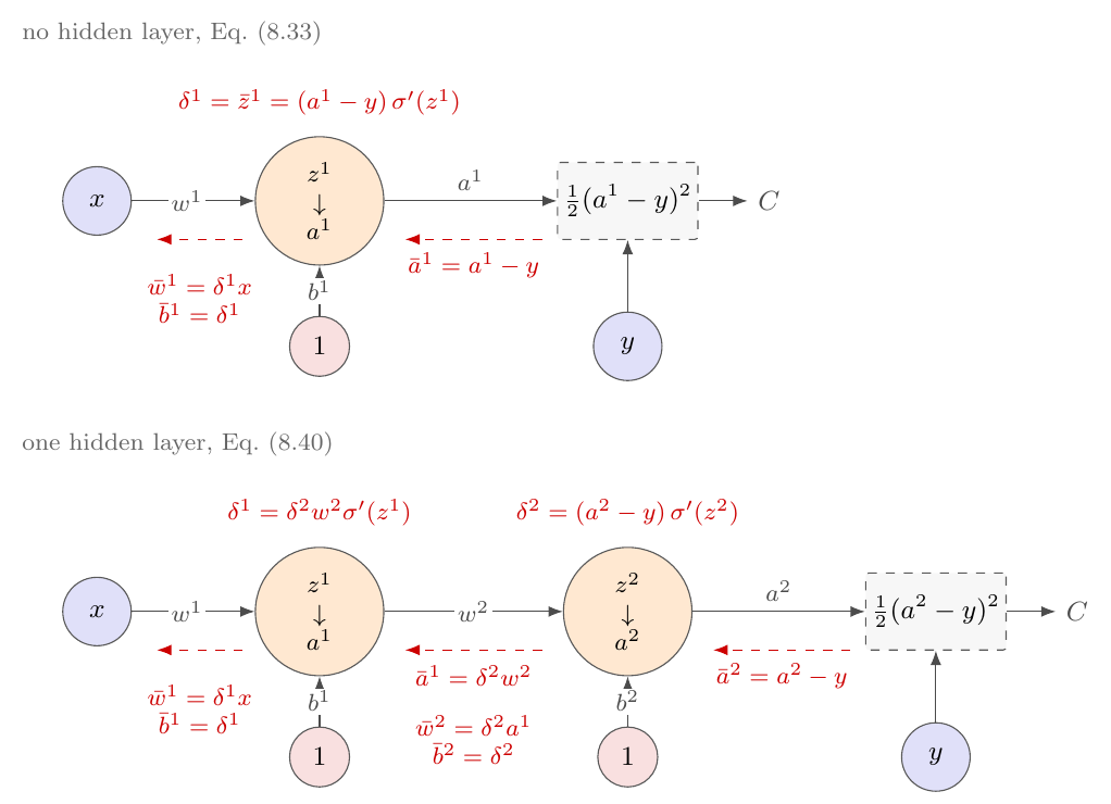
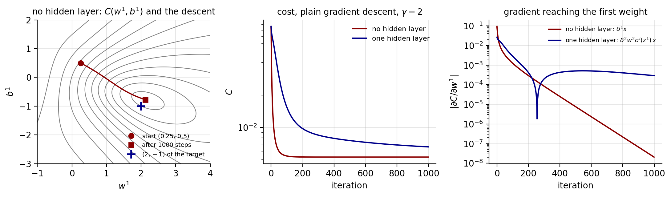
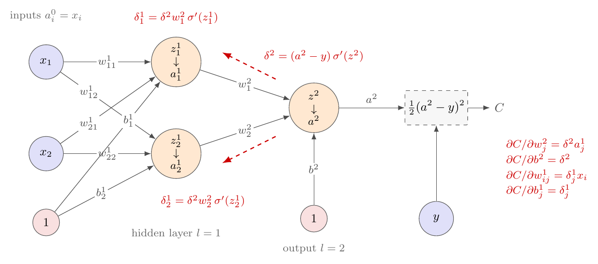
That we nonetheless train such networks successfully is an empirical fact rather than a theorem. Part of the explanation is that in high dimensions strict local minima are rare relative to saddle points, and that the many symmetric copies of a good solution make some good solution easy to reach.
8.8. Backpropagation#
We now derive the gradient. The derivation is short once the notation of
Section Notation and the feed-forward pass is in place, but the indices hide what is going
on, so we first work through the two smallest networks there are: a single
neuron with a scalar input and a scalar output, which is the logistic
regression of Figure 5.4 with a different loss, and the same
neuron with one hidden neuron in front of it, first by hand and then with
jax.grad. A third example, with two inputs and two hidden nodes,
then shows where the indices go. Everything that
Section The general case: dense layers does with matrices and sums, these
examples do with a handful of products, and the second of them already
contains the backpropagation equation.
8.8.3. The general case: dense layers#
Everything follows from the chain rule (1.51) and from two elementary derivatives of Eq. (8.18),
together with the derivative of the activation, \(\partial a_j^{l}/\partial z_j^{l}=f'(z_j^{l})\), which for the sigmoid is \(a_j^{l}(1-a_j^{l})\) by Eq. (8.22).
The output layer.
Take the squared-error cost (8.32) and specialise to \(l=L\). Differentiating with respect to a weight in the last layer,
The structure of the result invites a definition. Introduce the error of node \(j\) in the output layer,
where \(\circ\) is the Hadamard product of Section Vectors. With it, Eq. (8.58) becomes simply
Equation (8.59) is worth reading rather than merely recording. The second factor measures how fast the cost changes with the \(j\)th output: if the cost hardly depends on output \(j\), then \(\delta_j^{L}\) is small, which is what one would want. The first factor measures how fast the activation function is changing at the value \(z_j^{L}\) actually attained: a saturated unit, with \(f'\approx0\), contributes almost nothing however wrong it is. That second observation is the seed of the vanishing-gradient problem.
The error is the bias gradient. Note that \(\delta_j^{L}\) can be written as
and since \(\partial z_j^{L}/\partial b_j^{L}=1\) from Eq. (8.18),
The error of a node is the derivative of the cost with respect to that node’s bias. This is not a coincidence but a consequence of the bias entering \(z\) additively, and it is why the same symbol serves both purposes.
Propagating the error backwards. It remains to obtain \(\bm{\delta}^{l}\) for a general layer. Define \(\delta_j^{l}=\partial C/\partial z_j^{l}\) as before, and express it through the layer above. Since \(C\) depends on \(z_j^{l}\) only through the activations \(z_k^{l+1}\) of the next layer, the chain rule gives
From \(z_k^{l+1}=\sum_i w_{ik}^{l+1}a_i^{l}+b_k^{l+1}\) and \(a_i^{l}=f(z_i^{l})\) we obtain \(\partial z_k^{l+1}/\partial z_j^{l}=w_{jk}^{l+1}f'(z_j^{l})\), and therefore
This is the backpropagation equation. The error at a layer is the error at the layer above, pulled back through the transpose of the weights and modulated by the local derivative of the activation. Figure 8.13 draws it next to the forward pass of Figure 8.6: the same graph, the same weights, the arrows reversed.
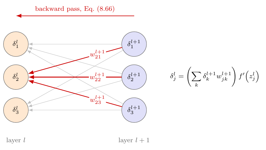
Figure 8.13: The backward pass of Eq. (8.64), drawn on the same network as Fig. 8.6 but with the arrows reversed. The error \(\delta_j^{l}\) of node \(j\) in layer \(l\) receives a contribution from every node \(k\) of layer \(l+1\), weighted by the same \(w_{jk}^{l+1}\) that carried \(a_j^{l}\) forward, and the sum is then modulated by the local derivative \(f'(z_j^{l})\). Comparing with Fig. 8.6 shows what backpropagation is: the identical graph traversed in the opposite direction, with the transpose of each weight matrix in place of the matrix itself. A saturated node, one with \(f'(z_j^{l})\approx0\), blocks the flow entirely, which is the mechanism of Section Vanishing and exploding gradients.
8.8.4. The four equations of backpropagation#
Collecting the results gives the four equations on which everything rests:
Equation (8.65) starts the recursion at the output, (8.66) carries it backwards through the network, and (8.67) and (8.68) convert the errors into the gradients we actually want. Every quantity on the right is already available: the \(\bm{z}^{l}\) and \(\bm{a}^{l}\) were computed during the forward pass and need only be stored, and \(f'\) is a cheap element-wise function.
A simplification worth knowing. For the two natural pairings of output activation and loss, the first equation collapses. With a linear output layer and the half-squared error (8.32), \(f'=1\) and \(\partial C/\partial a_j^{L}=a_j^{L}-y_j\), so
With a softmax output and the multiclass cross entropy (5.28), the derivative of the softmax and the derivative of the logarithm cancel – the same cancellation met in the notebox of Section Maximum likelihood and the cross-entropy – and Eq. (8.69) holds again. In both cases the output error is simply prediction minus target, with no factor of \(f'\) to shrink it. This is the deeper reason for pairing the softmax with the cross entropy, and it is why the implementation of Section A neural network from scratch treats both heads with one line of code.
Cost.
Counting operations, Eq. (8.66) costs one matrix-vector product per layer, exactly as the forward pass does. The whole gradient with respect to all parameters therefore costs about twice a forward pass, independently of the number of parameters. This is precisely the claim made for reverse-mode automatic differentiation in Section Automatic differentiation, and backpropagation is that algorithm specialised to a layered network. Computing the same gradient by finite differences, Eq. (4.102), would require one forward pass per parameter; for a network with \(10^{6}\) weights the difference is between a second and a fortnight.
8.8.5. The algorithm#
Putting it together, training a feed-forward network proceeds as follows.
Set-up.
Fix the architecture: the number of inputs and outputs, the number of hidden layers and the number of nodes in each.
Choose activation functions for the hidden layers and for the output layer, the latter dictated by the range of the target.
Choose the cost function, again dictated by the distribution of the target, and any regularisation terms with their hyperparameters.
Choose the optimiser from Chapter 4 – plain gradient descent, momentum, RMSProp, Adam – and its learning rate.
Initialise the weights and biases, as discussed in Section Weight initialisation.
Each iteration.
Forward pass. Set \(\bm{a}^{0}=\bm{x}\) and compute \(\bm{z}^{l}\) and \(\bm{a}^{l}=f(\bm{z}^{l})\) for \(l=1,2,\dots,L\) by Eq. (8.20), storing every \(\bm{z}^{l}\) and \(\bm{a}^{l}\).
Output error. Compute \(\bm{\delta}^{L}\) from Eq. (8.65), or from Eq. (8.69) for the natural pairings.
Backward pass. For \(l=L-1,L-2,\dots,1\) compute \(\bm{\delta}^{l}\) from Eq. (8.66).
Gradients. Form \(\partial C/\partial w_{ij}^{l}=\delta_j^{l}a_i^{l-1}\) and \(\partial C/\partial b_j^{l}=\delta_j^{l}\).
Update. With plain gradient descent and learning rate \(\gamma\),
\[ w_{ij}^{l}\leftarrow w_{ij}^{l}-\gamma\,\delta_j^{l}a_i^{l-1}, \qquad b_j^{l}\leftarrow b_j^{l}-\gamma\,\delta_j^{l},\tag{8.70} \]or substitute any of the schemes of Chapter 4.
In practice steps 1–5 are applied to a minibatch rather than a single sample, as in Section Stochastic gradient descent, and one pass over all minibatches is an epoch.
Machine learning connection
Always verify a hand-written backpropagation implementation against finite differences before trusting it. Perturb one weight by \(h\approx10^{-6}\), evaluate the cost twice, and compare the central difference (4.102) with the analytical gradient; the relative discrepancy should be around \(10^{-6}\) or smaller. A wrong gradient does not usually announce itself – the network still trains, just to the wrong place, or trains slightly worse than it should – and this check takes minutes to write. The implementation of Section A neural network from scratch passes it at \(10^{-6}\) to \(10^{-8}\) for every activation function and both output heads, and those numbers are quoted there precisely so that a reader reimplementing it has something to compare against.
8.9. Vanishing and exploding gradients#
Backpropagation as derived above is correct, and for deep networks it does not work. Understanding why occupied the field for two decades and the explanation is contained in Eq. (8.66).
Unrolling the recursion from the output down to layer \(l\),
so the gradient reaching layer \(l\) is a product of \(L-l\) factors. A product of many numbers each smaller than one shrinks geometrically; a product of many numbers each larger than one grows geometrically. Neither behaviour is survivable.
In the first case the gradients reaching the early layers are so small that gradient descent leaves those weights essentially unchanged, and training never converges to a good solution. This is the vanishing gradients problem. In the second the updates are so large that the iteration diverges: the exploding gradients problem, encountered particularly in recurrent networks where the same weight matrix is applied at every time step. More generally, deep networks suffer from unstable gradients, with different layers learning at widely different speeds.
The sigmoid is the principal culprit. Consider the factors in Eq. (8.71) for the logistic activation. By Eq. (8.22) the derivative \(\sigma'\) never exceeds \(\tfrac14\), and it approaches zero rapidly once \(|z|\) is large, so a saturated unit contributes almost nothing. Even in the best case, with every unit at its most sensitive, ten layers multiply ten factors of at most \(\tfrac14\), giving \(4^{-10}\approx10^{-6}\): the first layer receives a gradient a millionth of the size of the last. Sigmoid networks of any depth are, by construction, almost untrainable at their input end.
Glorot and Bengio identified a second contribution in 2010. With the then standard initialisation – weights drawn from \(\mathcal{N}(0,1)\) – the variance of the outputs of each layer is considerably larger than the variance of its inputs. Going forward through the network the variance grows layer by layer until the activations saturate at the top, and a saturated activation has a vanishing derivative. The logistic function makes matters worse still by having mean \(\tfrac12\) rather than zero, which is why \(\tanh\), with mean zero, behaves noticeably better in deep networks.
The two repairs. The first is the activation function. ReLU does not saturate for positive arguments and its derivative is exactly \(1\) there, so the factors in Eq. (8.71) do not shrink the gradient at all along the active path. This single change is most of the reason deep networks became trainable, and the ReLU family of Section Activation functions is the standard choice for that reason rather than for any biological one.
The second is initialisation, and it is the subject of the next section.
Figure 8.14 measures the effect directly. For each network the Frobenius norm of the weight gradient is plotted layer by layer after a single backward pass. With sigmoid activations the norm falls by orders of magnitude from the output towards the input, and the deeper the network the more severe the attenuation – at eight hidden layers the first layer receives a gradient several orders of magnitude smaller than the last, so it is effectively frozen. With ReLU the profile is far flatter and the early layers continue to receive a usable signal. This is Eq. (8.71) made visible.
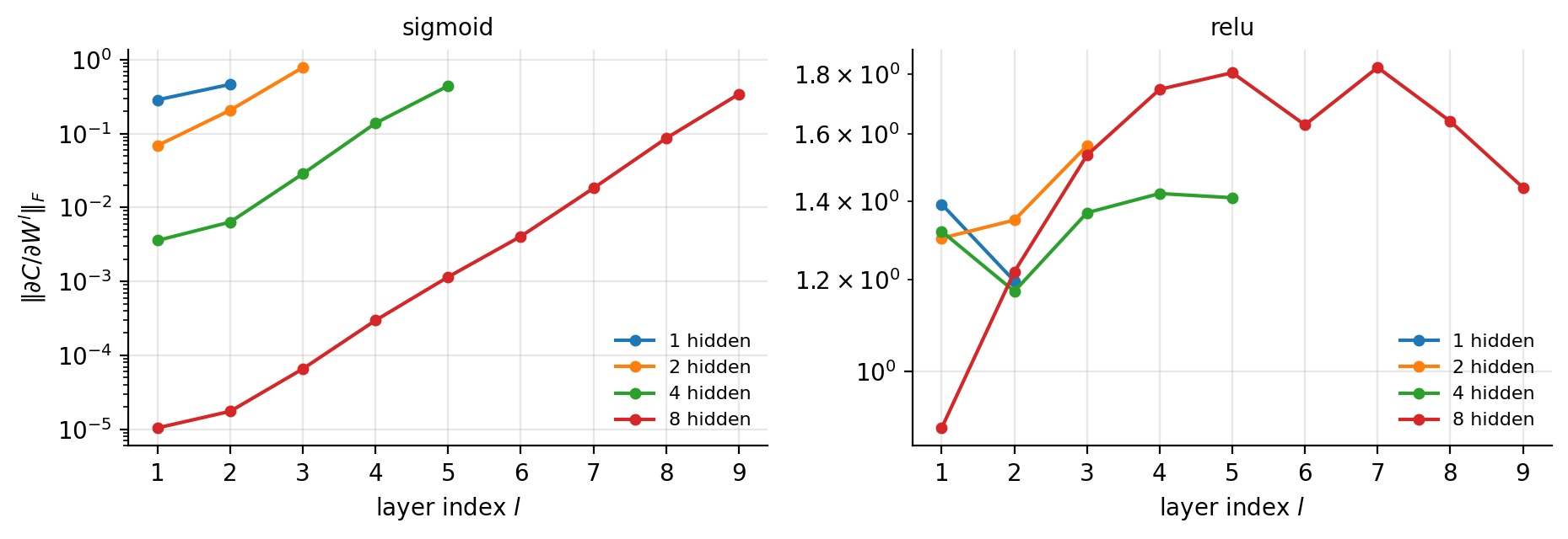
Figure 8.14: Norm of the weight gradient at each layer after one backward pass, for networks of \(1\), \(2\), \(4\) and \(8\) hidden layers of \(30\) units on the digits data. Left: sigmoid activations, showing severe attenuation towards the input. Right: ReLU, which preserves the gradient far better.
8.10. Weight initialisation#
The argument of Glorot and Bengio is that for a signal to propagate properly we need the variance of the outputs of each layer to equal the variance of its inputs in the forward direction, and the variance of the gradients to be preserved in the backward direction.
Suppose the inputs to a layer are independent with variance \(\var(a)\), and the \(M_{l-1}\) weights are independent with mean zero and variance \(\var(w)\). Then by the rules of Section Expectation values and moments, the activation \(z_j=\sum_i w_{ij}a_i\) has variance
so \(\var(z)=\var(a)\) requires \(\var(w)=1/M_{l-1}\). Repeating the argument for the backward pass, where Eq. (8.66) sums over the \(M_l\) nodes of the next layer, gives \(\var(w)=1/M_l\). The two conditions cannot both hold unless the layers have equal width, and Xavier or Glorot initialisation compromises between them,
drawing the weights from a Gaussian or a uniform distribution with this variance.
For ReLU the argument needs one correction. Since ReLU zeroes half of its inputs on average, it halves the variance, and compensating for this gives He initialisation,
which is the appropriate choice for the whole ReLU family. Biases are initialised to zero, or to a small positive constant such as \(0.01\) when using ReLU, so that units start on the active side of the kink.
It is worth appreciating how much rests on Eq. (8.72). Initialising all weights to zero would make every unit in a layer compute the same thing and receive the same gradient, so they would remain identical forever – the symmetry of Section The cost function and the optimisation problem must be broken by the initialisation. Initialising them too large saturates the activations; too small and the signal dies out. The permissible window is narrow, and Eqs. (8.73) and (8.74) locate it.
8.11. Classification with neural networks#
Classification requires only that the output layer and the loss be chosen correctly, and both were determined in Chapter 5.
For \(K\) classes the output layer has \(K\) nodes and the softmax activation (5.27),
so that the outputs are non-negative and sum to one and may be read as class probabilities. As in Section More than two classes: the softmax the exponentials must be computed after subtracting the largest score, Eq. (5.30), or they overflow. The loss is the multiclass cross entropy (5.28) with one-hot targets, and by the cancellation noted after Eq. (8.69) the output error is simply \(\bm{\delta}^{L}=\bm{a}^{L}-\bm{y}\).
The whole apparatus therefore reduces to multinomial logistic regression applied to the learned features \(\bm{a}^{L-1}\) rather than to the raw inputs. A classification network is Chapter 5 with a representation learner bolted on in front, and this is the most useful way to think about what the hidden layers are for.
8.12. Regularisation and hyperparameters#
A network with more parameters than data points can fit the training set exactly, so the bias-variance considerations of Section The bias-variance tradeoff apply with full force and some form of control is essential.
Weight penalties. Adding \(\lambda\|\bm{\Theta}\|_2^{2}\) to Eq. (8.31) is the Ridge penalty of Section Ridge regression under the name weight decay; it contributes \(2\lambda\bm{W}^{l}\) to each weight gradient and nothing to the bias gradients, since biases are not penalised for the reason given in Section Scaling, centring and the intercept. An \(\ell_1\) penalty produces sparse weights exactly as in Section The Lasso.
Early stopping. Monitor the cost on a validation set and stop when it begins to rise while the training cost still falls. This is the criterion of Section Learning rate schedules and stopping, and for networks it is the single most effective and cheapest regulariser available.
Dropout. During training, delete each unit independently with probability \(p\), typically \(0.5\) for hidden layers, and rescale the survivors; at test time use the whole network. Each minibatch therefore trains a different thinned network, and the final model behaves like an average over exponentially many of them – which is the variance reduction of Section Why averaging helps obtained without training an ensemble. Dropout also prevents units from co-adapting, since no unit can rely on any particular other unit being present.
Batch normalisation. Normalise the activations of a layer across the minibatch to zero mean and unit variance, then rescale by two learned parameters. This keeps the inputs of each layer in the well-behaved region of its activation function and hence attacks the vanishing-gradient problem directly; it also acts as a mild regulariser, since the statistics depend on the composition of the minibatch. The connection to Section The learning rate and the condition number is exact: standardising the inputs to a layer improves the conditioning of the optimisation problem that layer poses, and Eq. (4.26) says what that is worth.
Gradient clipping. If the gradient norm exceeds a threshold, rescale it to that threshold. This does not cure exploding gradients but it prevents a single bad minibatch from destroying the parameters, and it is standard practice in recurrent networks.
Hyperparameters. The number of hidden layers and their widths, the learning rate and its schedule, the batch size, \(\lambda\), the dropout rate and the activation function are all hyperparameters, and they are chosen by the cross-validation of Section Cross-validation on a validation set – never on the test set. Two rules of thumb survive contact with practice: the learning rate is by far the most important, and it is usually better to build a network somewhat too large and regularise it than to search for exactly the right size.
8.13. A neural network from scratch#
We now implement the whole of Sections Notation and the feed-forward pass to Weight initialisation. The code follows the equations line for line, uses the batched form (8.21) so that samples are rows throughout, and handles both regression and classification.
import numpy as np


def sigmoid(z):
    """Numerically stable logistic function, Eq. (8.sigmoid)."""
    out = np.empty_like(z, dtype=float)
    p, n = z >= 0, z < 0
    out[p] = 1.0 / (1.0 + np.exp(-z[p]))
    e = np.exp(z[n]); out[n] = e / (1.0 + e)
    return out

def sigmoid_prime(z):  s = sigmoid(z); return s * (1 - s)
def relu(z):           return np.maximum(0.0, z)            # Eq. (8.relu)
def relu_prime(z):     return (z > 0).astype(float)
def leaky_relu(z, a=0.01):        return np.where(z > 0, z, a * z)
def leaky_relu_prime(z, a=0.01):  return np.where(z > 0, 1.0, a)
def elu(z, a=1.0):                                          # Eq. (8.elu)
    return np.where(z > 0, z, a * (np.exp(np.minimum(z, 0)) - 1))
def elu_prime(z, a=1.0):
    return np.where(z > 0, 1.0, a * np.exp(np.minimum(z, 0)))
def tanh_(z):          return np.tanh(z)
def tanh_prime(z):     return 1 - np.tanh(z)**2
def identity(z):       return z
def identity_prime(z): return np.ones_like(z)

def softplus(z):       return np.log1p(np.exp(-np.abs(z))) + np.maximum(z, 0)
def softplus_prime(z): return sigmoid(z)

def gelu(z):
    """Exact GELU, Eq. (8.gelu); erf comes from scipy."""
    from scipy.special import erf
    return z * 0.5 * (1.0 + erf(z / np.sqrt(2.0)))

def gelu_prime(z):
    from scipy.special import erf
    Phi = 0.5 * (1.0 + erf(z / np.sqrt(2.0)))
    phi = np.exp(-0.5 * z**2) / np.sqrt(2.0 * np.pi)      # the normal density
    return Phi + z * phi                                   # d/dz [z Phi(z)]

def gelu_tanh(z):
    """The approximation of Eq. (8.geluapprox) used by most frameworks."""
    return 0.5 * z * (1 + np.tanh(np.sqrt(2 / np.pi) * (z + 0.044715 * z**3)))

def swish(z):          return z * sigmoid(z)               # Eq. (8.swish)
def swish_prime(z):
    s = sigmoid(z); return s + z * s * (1 - s)

def mish(z):                                               # Eq. (8.mish)
    sp = np.log1p(np.exp(-np.abs(z))) + np.maximum(z, 0)
    return z * np.tanh(sp)

def mish_prime(z, h=1e-6):
    return (mish(z + h) - mish(z - h)) / (2 * h)           # numerical is adequate

def softmax(z):
    """Eq. (8.softmax), with the shift of Eq. (5.softmaxstable)."""
    e = np.exp(z - np.max(z, axis=1, keepdims=True))
    return e / np.sum(e, axis=1, keepdims=True)

ACT = {"sigmoid": (sigmoid, sigmoid_prime), "relu": (relu, relu_prime),
       "leaky_relu": (leaky_relu, leaky_relu_prime), "elu": (elu, elu_prime),
       "tanh": (tanh_, tanh_prime), "identity": (identity, identity_prime),
       "softplus": (softplus, softplus_prime), "gelu": (gelu, gelu_prime),
       "swish": (swish, swish_prime), "mish": (mish, mish_prime)}
The network itself is short. Note in particular _backward, which is
Eqs. (8.65)–(8.68) transcribed.
class NeuralNetwork:
    """Fully connected feed-forward network trained by backpropagation.

    layer_sizes : e.g. [64, 50, 10] for 64 inputs, one hidden layer of 50
                  units and 10 outputs.
    task        : "classification" (softmax + cross entropy) or
                  "regression" (linear output + half-squared error).
    """

    def __init__(self, layer_sizes, hidden_activation="sigmoid",
                 task="classification", gamma=0.1, lmbd=0.0, epochs=100,
                 batch_size=32, rng=None):
        self.sizes, self.task = layer_sizes, task
        self.f, self.fp = ACT[hidden_activation]
        self.gamma, self.lmbd = gamma, lmbd
        self.epochs, self.batch = epochs, batch_size
        self.rng = np.random.default_rng(0) if rng is None else rng
        self._init_parameters(hidden_activation)

    def _init_parameters(self, act):
        """Xavier (8.xavier) or He (8.he) initialisation, by activation."""
        self.W, self.b = [], []
        for i in range(len(self.sizes) - 1):
            nin, nout = self.sizes[i], self.sizes[i + 1]
            s = np.sqrt(2.0 / nin) if act in ("relu", "leaky_relu", "elu") \
                else np.sqrt(1.0 / nin)
            self.W.append(self.rng.normal(0, s, (nin, nout)))
            self.b.append(np.zeros(nout) + 0.01)

    def _forward(self, X):
        """Eq. (8.forwardbatch); keeps every z and a for the backward pass."""
        a, z = [X], []
        for l in range(len(self.W)):
            zl = a[-1] @ self.W[l] + self.b[l]
            z.append(zl)
            if l == len(self.W) - 1:
                a.append(softmax(zl) if self.task == "classification" else zl)
            else:
                a.append(self.f(zl))
        return a, z

    def _backward(self, X, Y):
        """The four equations (8.bp1)-(8.bp4)."""
        n = X.shape[0]
        a, z = self._forward(X)

        # With softmax + cross entropy, and with a linear output under the
        # half-squared error, the output error is the same expression:
        delta = (a[-1] - Y) / n                       # Eq. (8.deltaLsimple)

        gW, gb = [None] * len(self.W), [None] * len(self.b)
        for l in range(len(self.W) - 1, -1, -1):
            gW[l] = a[l].T @ delta + self.lmbd * self.W[l]   # Eq. (8.bp4)
            gb[l] = np.sum(delta, axis=0)                    # Eq. (8.bp3)
            if l > 0:
                delta = (delta @ self.W[l].T) * self.fp(z[l - 1])  # Eq. (8.bp2)
        return gW, gb

    def fit(self, X, y):
        X = np.asarray(X, dtype=float)
        if self.task == "classification":
            self.classes_ = np.unique(y)
            idx = {c: i for i, c in enumerate(self.classes_)}
            Y = np.zeros((len(y), len(self.classes_)))        # one-hot
            Y[np.arange(len(y)), [idx[c] for c in y]] = 1
        else:
            Y = np.asarray(y, dtype=float).reshape(-1, 1)

        n = X.shape[0]
        self.loss_ = []
        for _ in range(self.epochs):
            order = self.rng.permutation(n)                   # shuffle, Sec. 4.practicaltips
            for s in range(0, n, self.batch):
                b = order[s:s + self.batch]
                gW, gb = self._backward(X[b], Y[b])
                for l in range(len(self.W)):                  # Eq. (8.update)
                    self.W[l] -= self.gamma * gW[l]
                    self.b[l] -= self.gamma * gb[l]
            self.loss_.append(self.cost(X, Y))
        return self

    def cost(self, X, Y):
        o = self._forward(X)[0][-1]
        if self.task == "classification":
            return float(-np.mean(np.sum(Y * np.log(np.clip(o, 1e-12, 1)), axis=1)))
        return float(0.5 * np.mean((o - Y)**2))               # Eq. (8.mse)

    def predict_proba(self, X):
        return self._forward(np.asarray(X, dtype=float))[0][-1]

    def predict(self, X):
        o = self.predict_proba(X)
        return (self.classes_[np.argmax(o, axis=1)]
                if self.task == "classification" else o.ravel())
Verifying the gradient.
Before using the network for anything we check _backward against
finite differences, as urged in the notebox of
Section The algorithm.
def gradient_check(net, X, Y, h=1e-6, n_samples=15):
    """Compare backpropagation with the central difference (4.gradcheck)."""
    rng = np.random.default_rng(0)
    gW, gb = net._backward(X, Y)
    worst = 0.0
    for l in range(len(net.W)):
        for _ in range(n_samples):
            i = rng.integers(net.W[l].shape[0]); j = rng.integers(net.W[l].shape[1])
            net.W[l][i, j] += h; c1 = net.cost(X, Y)
            net.W[l][i, j] -= 2 * h; c2 = net.cost(X, Y)
            net.W[l][i, j] += h
            num = (c1 - c2) / (2 * h)
            worst = max(worst, abs(num - gW[l][i, j])
                        / (abs(num) + abs(gW[l][i, j]) + 1e-12))
    return worst
Run over a three-hidden-layer network for every activation function, and over regression as well as classification heads, the worst relative discrepancy is
classification, sigmoid                     1.38e-06
classification, tanh                        1.11e-08
classification, relu                        4.46e-07
classification, leaky_relu                  5.80e-07
classification, elu                         2.08e-08
classification, softplus                    1.48e-06
classification, gelu                        3.25e-07
classification, swish                       3.33e-08
classification, mish                        7.29e-08
regression, tanh                            3.55e-08
regression, relu, 2 hidden layers           1.19e-08
which is the accuracy of the difference scheme itself. The implementation of Eqs. (8.65)–(8.68) is correct.
8.14. Examples#
Handwritten digits.
The digits data set bundled with scikit-learn contains \(1797\) images
of \(8\times8\) pixels, giving \(64\) inputs and \(10\) classes. We standardise the
features as urged in Section Arrays in practice: numpy, BLAS and LAPACK, hold out a fifth for testing,
and train a network with a single hidden layer of \(50\) units.
import numpy as np
from sklearn.datasets import load_digits
from sklearn.model_selection import train_test_split
from sklearn.preprocessing import StandardScaler

digits = load_digits()
X = StandardScaler().fit_transform(digits.data)
X_train, X_test, y_train, y_test = train_test_split(X, digits.target,
                                                    test_size=0.2, random_state=42)

for activation in ["sigmoid", "relu"]:
    net = NeuralNetwork([64, 50, 10], activation, "classification",
                        gamma=0.1, lmbd=1e-4, epochs=60, batch_size=32,
                        rng=np.random.default_rng(2024)).fit(X_train, y_train)
    print(f"{activation:8s}: train {np.mean(net.predict(X_train) == y_train):.4f}  "
          f"test {np.mean(net.predict(X_test) == y_test):.4f}  "
          f"final loss {net.loss_[-1]:.4f}")
sigmoid : train 0.9937  test 0.9722  final loss 0.0585
relu    : train 1.0000  test 0.9722  final loss 0.0059
For comparison, sklearn.neural_network.MLPClassifier with the same
architecture reaches \(0.9778\) on the same split. Our implementation is within
one test sample of a mature library, which is the appropriate standard.
The two activations reach the same test accuracy by different routes. ReLU drives the training loss an order of magnitude lower and fits the training set exactly, while the sigmoid does not; that the test accuracies coincide means the extra fitting bought nothing, which is the bias-variance story of Section The bias-variance tradeoff in a network. With only one hidden layer the vanishing-gradient argument of Section Vanishing and exploding gradients has little room to operate; its consequences appear when the depth grows, which is the subject of one of the exercises.
Figure 8.15 shows the training curves and the effect of capacity. On the left, ReLU drives the training cross entropy roughly an order of magnitude below the sigmoid within sixty epochs, and \(\tanh\) falls between them – the ordering the derivatives of Figure 8.9 predict. The test accuracies quoted in the legend are nevertheless within one sample of one another, which is the reminder that a lower training loss is not the objective. On the right, accuracy against the number of hidden units shows the familiar shape: rapid improvement up to about twenty units, then a plateau on the test set while the training accuracy continues to unity. The gap between the two curves is the variance term of Eq. (2.52).
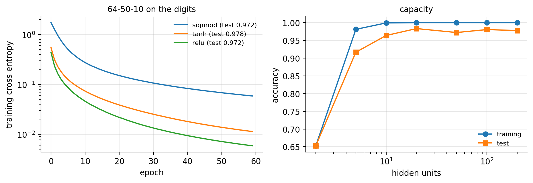
Figure 8.15: Left: training cross entropy against epoch for three hidden activations on the digits data, with the resulting test accuracies. Right: training and test accuracy against the width of the single hidden layer.
Using established libraries.
For anything beyond a teaching example one uses a framework, which supplies
automatic differentiation, GPU execution and a large catalogue of layers. In
scikit-learn,
from sklearn.neural_network import MLPClassifier

mlp = MLPClassifier(hidden_layer_sizes=(50,), activation="relu",
                    alpha=1e-4, max_iter=500, random_state=1)
mlp.fit(X_train, y_train)
print(f"test accuracy {mlp.score(X_test, y_test):.4f}")
and in PyTorch, where the correspondence with our equations is
visible:
import torch
import torch.nn as nn

model = nn.Sequential(nn.Linear(64, 50),   # Eq. (8.forwardbatch)
                      nn.ReLU(),           # Eq. (8.relu)
                      nn.Linear(50, 10))   # softmax folded into the loss
loss_fn = nn.CrossEntropyLoss()            # Eq. (5.multicrossentropy)
optimiser = torch.optim.Adam(model.parameters(), lr=1e-3)   # Sec. 4.adam

Xt = torch.tensor(X_train, dtype=torch.float32)
yt = torch.tensor(y_train, dtype=torch.long)
for epoch in range(100):
    optimiser.zero_grad()
    loss = loss_fn(model(Xt), yt)
    loss.backward()                        # this is Eqs. (8.bp1)-(8.bp4)
    optimiser.step()                       # this is Eq. (8.update)
The single call loss.backward() performs exactly the computation we
derived by hand, obtained by reverse-mode automatic differentiation over the
graph the forward pass recorded. Knowing what it does is the point of having
derived it.
8.15. Limitations, and a top-down view#
It is worth closing the exposition with some perspective, because the enthusiasm surrounding neural networks makes it easy to lose.
Deep networks are extraordinarily effective on data with strong local structure that can be exploited by an architecture – images, audio, text – and where very large labelled data sets exist. They are frequently not the best choice on the tabular data of Chapter 7, where gradient-boosted trees remain at least competitive and often better, while needing less tuning and no scaling. A network with no architectural prior adapted to the problem is a very flexible model with a great many hyperparameters, and flexibility is not free.
The specific limitations worth naming are these. Networks need large amounts of labelled data, and supervised deep learning has no good answer when labels are scarce. They are computationally expensive to train. They are largely uninterpretable: the variable-importance measures of Section Bagging have no clean analogue, and a network offers no account of why it predicted what it did. They extrapolate unpredictably outside the range of the training data. They are sensitive to adversarial perturbations imperceptible to a human. And the optimisation is non-convex, so results depend on initialisation and on the random seed, which makes honest reporting harder than for any method in the preceding chapters.
None of this argues against neural networks; it argues for choosing the method to suit the problem, which has been the theme of this book throughout. Section An extended example: learning the Ising energy makes the point with numbers: on the Ising chain a network can represent the answer exactly with \(2L\) hidden units and cannot find it from four hundred configurations, while the Lasso of Section The Lasso, given features a physicist chose, reaches \(R^{2}=0.99996\) on the same data.
8.16. An extended example: learning the Ising energy#
Section A second example: the one-dimensional Ising model fitted the energy of a one-dimensional Ising chain,
by linear regression, and the Lasso recovered it almost exactly. It did so because someone had first replaced the \(L\) spins by the \(L^{2}\) products \(s_js_k\), at which point Eq. (8.76) became a linear function of the inputs and the whole apparatus of Chapter 3 applied. The products were the physics. The regression only had to find which of them mattered.
This section removes that help. We hand a network the raw spins, with no products at all, and ask whether the interaction can be discovered. The example is a good closing test of the chapter because it separates three things that are easy to conflate: what a network can represent, what it can learn, and what it is worth relative to a linear model with well-chosen features. The answers here are, in order: everything, less than everything, and it depends entirely on how much data there is.
8.16.1. The linear model on raw spins is exactly powerless#
Before asking what the network gains, we should know what it is being compared against, and the answer is unusually clean.
Proposition 8.7 (The energy is uncorrelated with every spin)
Let the spins \(s_1,\dots,s_L\) be independent and uniform on \(\{-1,+1\}\) and let \(H\) be given by Eq. (8.76). Then \(\mathbb{E}\left[H\,s_j\right]=0\) for every \(j\), and the best linear predictor of \(H\) from \((s_1,\dots,s_L)\) is the constant \(\mathbb{E}[H]=0\).
Proof
Fix \(j\) and let \(T\) be the map that flips the \(j\)th spin, \(s_j\mapsto-s_j\), leaving the others alone. Since the spins are independent and uniform, \(T\) preserves the distribution. The energy contains \(s_j\) only through \(-J(s_{j-1}s_j+s_js_{j+1})\), and both terms change sign under \(T\); write \(H=A+B\) where \(B=-J(s_{j-1}s_j+s_js_{j+1})\) and \(A\) does not involve \(s_j\). Then
In the first term \(A\) and \(s_j\) are independent and \(\mathbb{E}[s_j]=0\), so it vanishes. In the second, \(Bs_j=-J(s_{j-1}+s_{j+1})\) after using \(s_j^{2}=1\), and \(\mathbb{E}[s_{j\pm1}]=0\), so it vanishes too. Since the covariance matrix of the spins is the identity, the least-squares coefficient vector is \(\mathbb{E}[H\bm{s}]=\bm{0}\). \qed
A linear model on raw spins is therefore not merely a weak model; it is provably equivalent to predicting the mean, and the same is true of Ridge and the Lasso, which can only shrink coefficients that are already zero in the population. Measured on the ten thousand configurations of Section A second example: the one-dimensional Ising model:
    max_j |corr(s_j, H)|                        : 0.0276
    max_j |mean(H s_j)|                         : 0.1748
    intercept                                   : +0.0395
    max_j |theta_j|                             : 0.1765
    R^2                                         : 0.004280
Four thousandths of the variance, which is sampling noise around the zero the proposition predicts. Note what this is not: it is not a statement that the energy is hard to compute from the spins. It is a deterministic function of them, computable in \(L\) multiplications. The information is entirely present and entirely invisible to any method that looks at one feature at a time. That is what a nonlinear model is for.
8.16.2. A network that gets it exactly right#
Section The universal approximation theorem showed that a one-hidden-layer network can approximate any continuous function on a compact set, and Theorem 8.2 quantified the width needed for a given accuracy. On this problem we can do better than approximate. The construction is short enough to write down.
Proposition 8.8 (An exact ReLU representation of the Ising energy)
For every \(L\) and every \(J\) there is a one-hidden-layer ReLU network with \(2L\) hidden units, all first-layer weights in \(\{-1,0,+1\}\) and all first-layer biases zero, that equals \(H(\bm{s})\) of Eq. (8.76) at every one of the \(2^{L}\) spin configurations. Explicitly,
Proof
For \(s,t\in\{-1,+1\}\) the sum \(s+t\) is \(\pm2\) when the spins agree and \(0\) when they differ, so \(|s+t|-1\) equals \(+1\) in the first case and \(-1\) in the second, which is exactly \(st\). Hence \(s_js_{j+1}=|s_j+s_{j+1}|-1\), and
Finally \(|z|=\sigma(z)+\sigma(-z)\), which turns each absolute value into two ReLU units, giving Eq. (8.78) with \(2L\) of them. The first-layer weight matrix has entries \(\pm1\) in two positions of each column and zero elsewhere; the output weights are all \(-J\) and the output bias is \(JL\). \qed
This is worth comparing with Section The universal approximation theorem in three ways. The representation is exact rather than approximate, because the input set is finite – the network need only agree with \(H\) on the corners of the hypercube, and Eq. (8.79) happens to be a piecewise-linear function that agrees everywhere in between as well. The width \(2L\) grows linearly in the input dimension rather than exponentially, because the target is a sum of terms each involving two coordinates; this is the same reason the Barron class of Theorem 8.3 escapes the curse of dimensionality, and \(H\) is a textbook member of it. And the ridge directions \(\pm(e_j+e_{j+1})\) are precisely the interactions we are trying to discover: reading the first-layer weights of Eq. (8.78) recovers the topology of the chain. Evaluating the hand-built network on all ten thousand configurations:
    hidden units                                : 80
    distinct first-layer weights                : [-1.0, 0.0, 1.0]
    max |network(s) - H(s)|                     : 0.000e+00
    R^2                                         : 1.0000000000
Zero error, not small error.
import numpy as np

# Proposition 8.isingexact, written down rather than trained
W1 = np.zeros((L, 2 * L))
for j in range(L):
    W1[j, 2 * j], W1[(j + 1) % L, 2 * j] = 1.0, 1.0        # +s_j + s_{j+1}
    W1[j, 2 * j + 1], W1[(j + 1) % L, 2 * j + 1] = -1.0, -1.0
W2, b2 = np.full(2 * L, -Jtrue), Jtrue * L
predict = lambda S: np.maximum(S @ W1, 0.0) @ W2 + b2
8.16.3. Representable is not learnable#
The network of Proposition 8.8 exists. Gradient descent has to find it, from the same \(400\) configurations Chapter 3 used, with no knowledge that the interaction is nearest-neighbour or even pairwise. One hidden layer, ReLU, mean squared error, Adam:
   epochs   R^2 train    R^2 test
       20    0.919057    0.187639
      100    1.000000    0.277651
      180    1.000000    0.277658
      260    1.000000    0.277658
      340    0.999990    0.282606
The training score reaches one after a hundred epochs and stays there; the test score reaches \(0.28\) and stops. This is overfitting in its purest form, and it is not cured by making the network bigger:
   hidden units   R^2 train    R^2 test
             10    0.957966   -0.599135
             25    1.000000   -0.055285
             50    1.000000    0.193549
            100    0.976503    0.185764
            200    0.999999    0.282703
            400    0.996122    0.315478
Width helps a little and monotonically, with no sign of the deterioration a naive reading of the bias-variance trade-off of Section The bias-variance tradeoff would predict – but \(400\) hidden units, five times the \(80\) that suffice for an exact fit, still reaches only \(0.32\). What is missing is data:
   training rows   R^2 test
             100   -0.213211
             200   -0.088174
             400    0.283759
             800    0.610756
            1600    0.875358
            3200    0.952438
and with enough of it the network does find something very close to the truth. Given \(8000\) configurations, \(400\) hidden units and \(1500\) epochs:
    R^2 train                                   : 0.998800
    R^2 test                                    : 0.980170
    RMS error in units of the energy quantum 2J : 0.4516
Figure 8.16 collects the three studies.
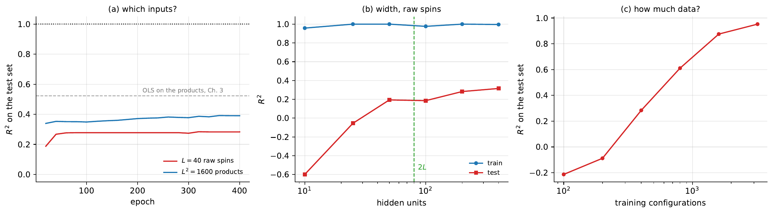
Figure 8.16: Learning the Ising energy with a one-hidden-layer network. (a) Test \(R^{2}\) against epoch for the \(L=40\) raw spins and for the \(L^{2}=1600\) products of Section A second example: the one-dimensional Ising model, both from \(400\) training configurations. (b) Width study on the raw spins; the dashed line marks the \(2L\) units that suffice for the exact representation of Proposition 8.8. (c) Test \(R^{2}\) against the number of training configurations: the limitation is data, not capacity.
The gap between \(R^{2}=1\), which a network of \(80\) units achieves with the right weights, and \(R^{2}=0.28\), which a network of \(200\) units achieves after being trained on \(400\) examples, is the whole distance between approximation theory and machine learning. Section The universal approximation theorem guarantees the former and says nothing at all about the latter. It is worth being explicit about why the guarantee is silent: the theorem quantifies over functions and asserts the existence of weights, whereas training is an optimisation over weights driven by a finite sample, and the sample is what fails here. With \(40\) inputs there are \(780\) pairwise interactions the network could believe in, and \(400\) configurations are not enough to rule out the \(740\) that are absent.
8.16.4. Against Chapter 3#
Now the comparison the section was built for. All models below are fitted on the same \(400\) configurations and scored on the same \(9600\) held-out ones.
   model                            R^2 on the 9600 test configurations
   OLS,   L^2 outer products              0.522863
   Ridge, L^2 outer products              0.522863
   Lasso, L^2 outer products              0.999963
   network, L^2 outer products            0.390631
   OLS,   L raw spins                    -0.112870
   network, L raw spins                   0.282703
   exact network, L raw spins             1.000000
Read from the bottom up. A network can be perfect and a linear model on the same inputs cannot do better than the mean – there is the case for nonlinearity, and it is absolute. Trained rather than constructed, the same network reaches \(0.28\), which is better than the linear model on the same inputs by an infinite margin and worse than the Lasso on engineered features by a wide one. And a network given the engineered features scores \(0.39\), below the \(0.52\) of plain OLS on those features and far below the Lasso: told that the answer is linear, the network still has to rediscover that fact from data, and it spends its capacity on a flexibility the problem does not need.
The ordering is uncomfortable if one expects networks to dominate, and it is the honest result. Its lesson is not that networks are weak. It is that in the regime \(n=400\), \(p=1600\), with a truth that is sparse in a known basis, a penalised linear model is the right tool, and the penalty of Section The Lasso encodes knowledge – most interactions are absent – that a network trained from scratch has to buy with data. Figure 8.17 shows the same numbers, together with the network’s score once it is given \(8000\) configurations instead of \(400\), which is where the ordering starts to reverse.
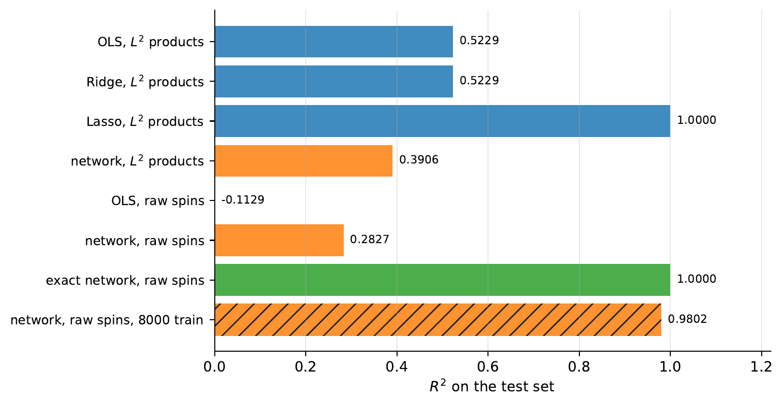
Figure 8.17: Every model of Section A second example: the one-dimensional Ising model and this section on the same problem. Blue: linear models. Orange: trained networks. Green: the exact network of Proposition 8.8. All bars use \(400\) training configurations and the same \(9600\) test configurations except the hatched one, which uses \(8000\) training configurations and a separate held-out set of \(2000\). Negative scores are drawn as zero and labelled.
The same experiment in PyTorch, with an independent initialisation and an independent shuffle, agrees:
   framework      R^2 train    R^2 test
   numpy           0.999999    0.282703
   PyTorch         0.996700    0.267799
import torch

model = torch.nn.Sequential(
    torch.nn.Linear(L, 200), torch.nn.ReLU(), torch.nn.Linear(200, 1)
).double()
opt = torch.optim.Adam(model.parameters(), lr=3e-3)
lossf = torch.nn.MSELoss()
for ep in range(400):
    perm = torch.randperm(ntr)
    for s in range(0, ntr, 40):
        b = perm[s:s + 40]
        opt.zero_grad()
        lossf(model(Xt[b]).squeeze(-1), yt[b]).backward()
        opt.step()
The two do not agree digit by digit and are not meant to. They agree on the conclusion, which is the only thing a cross-check can establish.
Machine learning connection
The exercise of this section – predicting the energy of a configuration of atoms or spins from the configuration alone – is the basis of machine-learned interatomic potentials, which are now a standard tool in computational chemistry and materials science. The economics are the same as here: a quantum-mechanical energy is expensive, a fitted surrogate is cheap, and the surrogate is only useful if it generalises to configurations never computed. Two features of the successful architectures are visible in miniature in Proposition 8.8. They are built from local terms – each hidden unit in Eq. (8.78) reads two neighbouring sites, not all forty – so the parameter count grows with the range of the interaction rather than the size of the system. And they enforce the symmetries of the problem by construction rather than learning them, which is exactly the data saving that Section Representable is not learnable shows is needed: our network had to spend thousands of configurations discovering that couplings beyond nearest neighbours are zero, whereas a locality constraint would have supplied that for free. Chapter 10 makes the same argument for images under translation, and it is the single most useful design principle in the subject.
8.17. Summary and the programs#
The chapter began with a promise made in Chapter 5: logistic regression is a neural network with no hidden layer. The XOR gate showed why that is not enough – a single layer computes a linear boundary, and linear regression on XOR returns the constant \(0.5\) while logistic regression achieves exactly chance – and a hidden layer of two units solved all three gates perfectly.
The mathematics is a composition. A layer computes \(\bm{z}^{l}=(\bm{W}^{l})^{T}\bm{a}^{l-1}+\bm{b}^{l}\) followed by an element-wise non-linearity; stacking layers gives the feed-forward pass, and the universal approximation theorem guarantees that one hidden layer suffices to represent any continuous function – while saying nothing about how many units are needed or whether gradient descent will find them.
The gradient follows from the chain rule alone, and
Sections Two scalar examples: no hidden layer and one hidden layer and Two inputs, two hidden nodes, one output worked it out
first on two scalar networks, by hand and with jax.grad, and on a
\(2\)–\(2\)–\(1\) network, where the reverse sweep of Section The same algorithm by automatic differentiation
continues through the hidden nodes. Defining the error
\(\delta_j^{l}=\partial C/\partial z_j^{l}\) gives the four
equations (8.65)–(8.68): the output error starts the
recursion, Eq. (8.66) pulls it backwards through the transposed
weights modulated by \(f'\), and the weight and bias gradients follow
immediately. The whole gradient costs about two forward passes regardless of
the number of parameters, which is reverse-mode automatic differentiation from
Section Automatic differentiation specialised to a layered graph. For the natural
pairings of output activation and loss – linear with squared error, softmax
with cross entropy – the output error collapses to
\(\bm{\delta}^{L}=\bm{a}^{L}-\bm{y}\).
Two practical problems then had to be solved before any of this worked in depth. Equation (8.71) shows the gradient reaching layer \(l\) to be a product of \(L-l\) factors, which shrinks or grows geometrically; since \(\sigma'\le\tfrac14\), a ten-layer sigmoid network attenuates the gradient by \(10^{-6}\) before it reaches the first layer. The repairs were the ReLU family, which does not saturate, and the variance-preserving initialisations of Eqs. (8.73) and (8.74).
The implementation of Section A neural network from scratch is those equations transcribed, and it was verified against finite differences to between \(10^{-6}\) and \(10^{-8}\) for every activation function and both output heads before being used on anything.
The complete programs are collected in doc/BookML/BookPrograms:
gates.py– linear regression, logistic regression and a neural network on the AND, OR and XOR gates of Table 8.1.neural_network.py– the activation functions and theNeuralNetworkclass of Section A neural network from scratch, with the gradient check.digits.py– the handwritten-digit example, the comparison againstscikit-learn, and the depth study used in the exercises.frameworks.py– the same network inscikit-learnandPyTorch.ising_network.py– the Ising study of Section An extended example: learning the Ising energy: the vanishing spin-energy correlation of Proposition 8.7, the exact \(2L\)-unit network of Proposition 8.8, width and sample-size studies, the comparison against the three estimators of Section A second example: the one-dimensional Ising model, and aPyTorchcross-check.
8.18. Exercises#
8.18.1. Warm-up exercises#
Linear layers collapse. (a) Show that a network with two layers and linear activations computes an affine function of its input, and identify the effective weight matrix and bias. (b) Deduce that depth is useless without a non-linearity. (c) Does the same argument apply if only the output layer is linear?
The XOR gate by hand. Construct explicitly a network with two inputs, two hidden units with the step activation and one output unit that computes XOR. Hint: let one hidden unit compute OR and the other NAND. Verify your weights on all four inputs.
Counting parameters. For an architecture \([M_0,M_1,\dots,M_L]\), show that the number of weights is \(\sum_l M_{l-1}M_l\) and the number of biases \(\sum_l M_l\). Evaluate both for \([64,50,10]\) and for \([784,300,100,10]\), and compare with the number of training samples in the digits and MNIST data sets respectively.
Derivatives of the activations. (a) Verify \(\sigma'=\sigma(1-\sigma)\) and \(\tanh'=1-\tanh^{2}\). (b) Show that \(\max_z\sigma'(z)=1/4\) and \(\max_z\tanh'(z)=1\). (c) Plot \(\sigma'\), \(\tanh'\), \(\mathrm{ReLU}'\) and \(\mathrm{ELU}'\) together and comment on which of them can attenuate a gradient.
Deriving the four equations. (a) Derive Eq. (8.59) from the squared-error cost. (b) Show that \(\delta_j^{l}=\partial C/\partial b_j^{l}\), Eq. (8.67). (c) Derive the recursion (8.66) using the chain rule, being explicit about why the sum over \(k\) appears. (d) Show that for a softmax output with the cross entropy the output error reduces to \(\bm{\delta}^{L}=\bm{a}^{L}-\bm{y}\).
The cost of the gradient. (a) Count the multiplications in one forward pass through \([M_0,\dots,M_L]\). (b) Count them in one backward pass, and show that the two are of the same order. (c) How many forward passes would a finite-difference gradient require? Evaluate for \([784,300,100,10]\) and comment.
Gradient check (numerical). Implement the network of Section A neural network from scratch and reproduce the gradient check. (a) Confirm a relative error around \(10^{-6}\) or smaller. (b) Deliberately introduce a bug – omit the \(f'(\bm{z}^{l})\) factor in Eq. (8.66) – and report what the check gives, and whether the network still trains. (c) Vary \(h\) from \(10^{-1}\) to \(10^{-12}\) and plot the discrepancy; explain the shape of the curve using the round-off discussion of Section Vector and matrix norms.
Vanishing gradients (numerical). Train networks of depth \(1,2,4,8\) hidden layers of \(30\) units each on the digits data, once with the sigmoid and once with ReLU. (a) For each, record the norm of the gradient at the first and the last hidden layer after one epoch. (b) Plot the ratio against depth and compare with the bound \(4^{-(L-1)}\) implied by Eq. (8.71). (c) Which activation permits training at depth eight?
Initialisation (numerical). (a) Initialise all weights to zero and explain, and then verify, what happens. (b) Compare \(\mathcal{N}(0,1)\), Xavier (8.73) and He (8.74) initialisation on a five-layer ReLU network, plotting the variance of the activations against layer index after one forward pass. (c) Relate what you see to Eq. (8.72).
Architecture and regularisation (numerical). On the digits data, sweep the number of hidden units from \(5\) to \(200\) and plot training and test accuracy. (a) Where does overfitting begin? (b) Add weight decay and repeat for several \(\lambda\). (c) Compare the best network with the random forest and the gradient-boosted trees of Chapter 7 on the same split, and with the logistic regression of Chapter 5. Comment on accuracy, training time and the number of hyperparameters each required.
8.18.2. Project-style exercise: building a neural network#
Part a: forward and backward. Implement a fully connected network from scratch, supporting an arbitrary list of layer sizes, a choice of hidden activation, and both output heads. Verify the gradient against finite differences for every activation and both heads, and report the worst relative error as a table. Do not proceed until this passes.
Part b: the gates. Reproduce Section Why one layer is not enough: the XOR problem: linear regression, logistic regression and your network on AND, OR and XOR. Then find the smallest hidden layer that solves XOR, and plot the decision boundary your network learns.
Part c: regression. Apply your network to the Franke function of Section A complete example: the Franke function with a linear output layer and the squared-error cost. Compare the test error against the OLS, Ridge and Lasso results of Chapter 3, at matched numbers of parameters where possible. Which method wins, and does the answer depend on the noise level?
Part d: classification. Apply it to the Wisconsin data of Section The Wisconsin breast cancer data and to the digits data. Report the metrics of Section Measuring the quality of a classifier on a test set used once. Compare against logistic regression, the support vector machine of Chapter 6 and the ensembles of Chapter 7.
Part e: optimisers and depth. Replace plain gradient descent by momentum, RMSProp and Adam from Chapter 4, sweeping the learning rate for each, and present the results as a table like Table 4.4. Then increase the depth and study the vanishing-gradient effect directly, comparing the sigmoid with ReLU.
Part f: regularisation. Add weight decay, early stopping and dropout, and quantify what each is worth on your hardest problem. Choose all hyperparameters by cross-validation on a validation set, and report a single number on the test set at the very end. Discuss honestly how much of the final performance came from the architecture and how much from the tuning.