
9. Chapter 9: Neural Networks for Differential Equations#
Chapter 8 built a neural network and trained it on labelled data. This chapter puts the same network to a different use: solving differential equations, where there are no labels at all. What replaces them is the equation itself. If we can write the residual of a differential equation as a function of the network and its derivatives, then driving that residual to zero is training, and the converged network is the solution.
The idea is due to Lagaris and collaborators in the 1990s and has been revived, under the name of physics-informed neural networks, as a large research area; a book-length treatment is given by Yadav and Kumar [yadav2015] and a recent survey by Cuomo and others [cuomo2022]. Our aim here is narrower and more concrete. We take the network of Section A neural network from scratch, extend it with the ability to differentiate its own output with respect to its input, and use it to solve four problems: exponential decay, logistic population growth, the one-dimensional Poisson equation, and then the diffusion and wave equations in one space dimension. At each stage we compare against the exact solution and against a classical numerical method, because a new method that is not compared against the old one has not been evaluated.
One thread from Chapter 8 becomes concrete here. The discussion of activation functions in Section Activation functions ended with the remark that the GELU family is the default choice for physics-informed networks because ReLU has no usable second derivative. In this chapter that remark stops being an aside: we shall see in Section Differentiating the network with respect to its input that a ReLU network has an identically zero second derivative and therefore cannot solve a second-order equation at all.
9.1. Ordinary differential equations#
An ordinary differential equation involves a function of one variable. In general it may be written
where \(g(x)\) is the function to be found and \(g^{(n)}\) its \(n\)-th derivative. The expression \(f\) is simply a way of writing that some relation among \(x\), \(g\) and its derivatives holds; the highest derivative appearing, \(n\), is the order of the equation. Equation (9.1) alone does not determine \(g\), and additional conditions – initial or boundary values – are required for the solution to be unique.
The trial solution. The central device is to write the candidate solution as
where \(N(x,P)\) is a neural network with parameters \(P\), the function \(h_1(x)\) alone makes \(g_t\) satisfy the required conditions, and \(h_2\) is constructed so that the network’s contribution vanishes wherever those conditions are imposed.
This construction is worth dwelling on, because it is what distinguishes the approach from simply adding the boundary conditions to the loss. The conditions are satisfied by construction, exactly, for any values whatever of the parameters, including the random values at initialisation. The optimiser is therefore never asked to trade accuracy at the boundary against accuracy in the interior; it has only one job, which is to make the equation hold. We shall see the consequence numerically: the error of our diffusion solution at \(t=0\) is exactly zero, to machine precision, at every stage of training.
The cost function. Equation (9.1) states that \(f\) should vanish. For a single input \(x\) we may therefore take the squared residual as the cost, and for \(N\) collocation points \(x_i\) the mean squared residual,
The network must find parameters \(P\) minimising Eq. (9.3).
Three remarks about this cost. It uses no labelled data: the \(x_i\) are points at which we choose to enforce the equation, not measurements, and they may be placed anywhere and changed at will. It is a mean squared error, so everything said in Section Deriving least squares from a probability distribution about squared losses applies, and the optimisation is that of Chapter 4 without modification. And it is emphatically not convex, so the warnings of Section The cost function and the optimisation problem apply with full force – a point we shall confirm the hard way in Section Exponential decay.
9.2. Differentiating the network with respect to its input#
Evaluating Eq. (9.3) requires derivatives of the network output with respect to its input. This is a different object from the gradients of Chapter 8, which were with respect to the parameters, and it is obtained by propagating derivatives forward through the layers rather than backwards.
Recall the feed-forward pass of Eq. (8.21), with \(\bm{a}^{0}=\bm{x}\),
with a linear output layer. Differentiating with respect to an input coordinate \(x_k\) and using the chain rule,
started from \(\partial\bm{a}^{0}/\partial x_k=\bm{e}_k\). Differentiating once more, and using the product rule on the second of Eqs. (9.5),
with \(\partial^{2}\bm{z}^{l}/\partial x_k^{2} =(\partial^{2}\bm{a}^{l-1}/\partial x_k^{2})\bm{W}^{l}\). These recursions run alongside the ordinary forward pass at a cost of one extra matrix product per layer per derivative order, so obtaining \(N\), \(N'\) and \(N''\) costs about three forward passes. This is forward-mode automatic differentiation, the counterpart of the reverse mode discussed in Section Automatic differentiation, and it is the efficient choice here precisely because the input is low-dimensional – one or two variables – whereas the parameters are many, which is why the parameter gradients still go backwards.
Why the activation function now matters more. Equation (9.6) requires \(f''\). This is where the choice of activation stops being a matter of taste. For the rectified family \(f''\equiv0\) wherever it is defined, and \(f'\) is piecewise constant, so every term in Eq. (9.6) vanishes: a ReLU network has an identically zero second derivative almost everywhere. It cannot represent the curvature that a second-order equation is about.
This is easily confirmed. Taking a network with two hidden layers of twenty units, initialised as in Section Weight initialisation, and evaluating \(\max|\partial^{2}N/\partial x^{2}|\) over a grid:
tanh         max|d2N/dx2| = 1.236e-01
gelu         max|d2N/dx2| = 1.014e+00
swish        max|d2N/dx2| = 6.354e-01
sigmoid      max|d2N/dx2| = 1.585e-02
softplus     max|d2N/dx2| = 2.386e-01
elu          max|d2N/dx2| = 1.385e+00
relu         max|d2N/dx2| = 0.000e+00
leaky_relu   max|d2N/dx2| = 0.000e+00
The two piecewise-linear activations give exactly zero, and every smooth activation gives something usable. The remark at the end of Section Which activation should we use? – that the GELU family is preferred wherever the network output must be differentiated – is this table. For the examples in this chapter we use \(\tanh\), which is smooth, bounded, and has the mild advantage over GELU of a derivative expressible in the function value; the exercises ask the reader to repeat the calculations with the others.
Figure 9.1 shows the same numbers on a logarithmic scale, where the two zeros can only be marked rather than plotted. The gap is not a matter of degree: the smooth activations differ among themselves by two orders of magnitude and all of them work, while the rectified ones are not small but identically zero and cannot work at all.
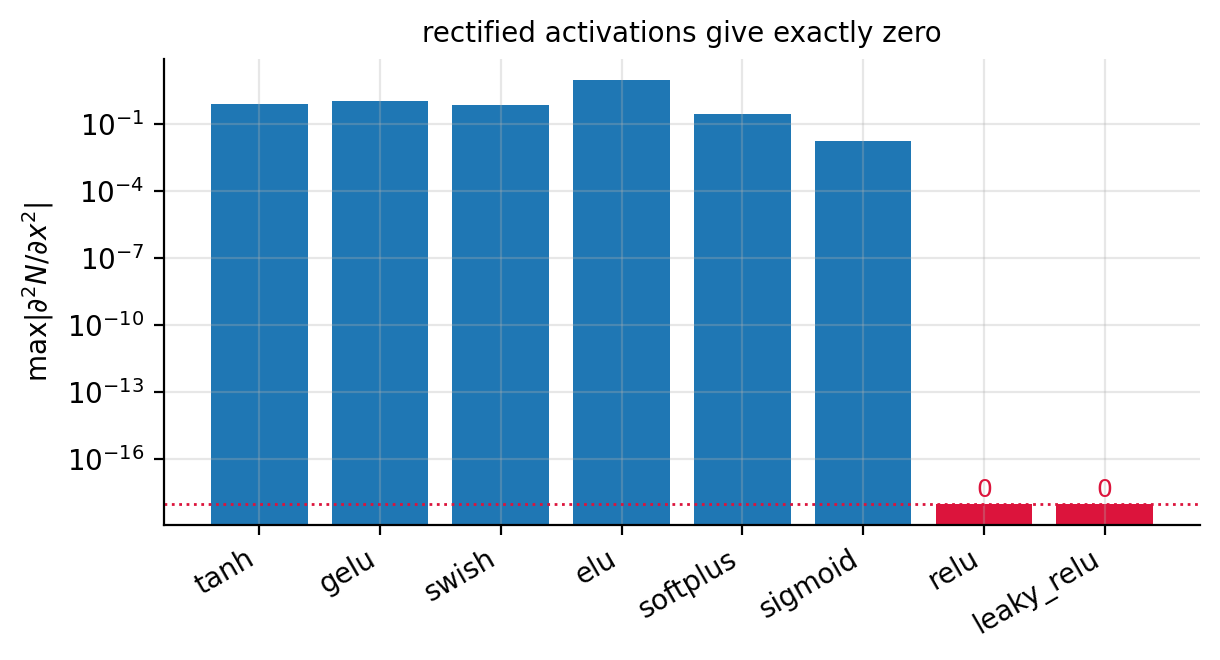
Figure 9.1: Largest second derivative of a randomly initialised network with two hidden layers of twenty units, by activation function. The rectified activations, in red, give exactly zero because \(f''\equiv0\) in Eq. (9.6).
Implementation. The recursions (9.5) and (9.6) are a direct transcription, and reuse the activation table of Section A neural network from scratch unchanged.
import autograd.numpy as np
from autograd import grad, elementwise_grad

def network(P, X, activation="tanh"):
    """Feed-forward pass, Eq. (8.forwardbatch), with a linear output layer."""
    f = ACT[activation]
    a = X
    for l, (W, b) in enumerate(P):
        z = a @ W + b
        a = f(z) if l < len(P) - 1 else z
    return a[:, 0]


def network_derivs(P, X, activation="tanh", order=2, k=0):
    """N, dN/dx_k and d2N/dx_k^2 by the forward recursions (9.firstderiv)
    and (9.secondderiv).  The activations and their derivatives are those
    of Section 8.nncode."""
    f = ACT[activation]
    fp = elementwise_grad(f)             # f'
    fpp = elementwise_grad(fp)           # f''

    a = X
    da = np.zeros_like(X) + (np.arange(X.shape[1]) == k)   # da0/dxk = e_k
    d2a = np.zeros_like(X)

    for l, (W, b) in enumerate(P):
        z, dz, d2z = a @ W + b, da @ W, d2a @ W
        if l < len(P) - 1:
            a, da, d2a = f(z), fp(z) * dz, fpp(z) * dz**2 + fp(z) * d2z
        else:                                              # linear output
            a, da, d2a = z, dz, d2z
    if order == 1:
        return a[:, 0], da[:, 0]
    return a[:, 0], da[:, 0], d2a[:, 0]
Checked against automatic differentiation of the same network, the analytic recursions agree to \(2\times10^{-16}\) in the first derivative and \(8\times10^{-17}\) in the second – that is, to machine precision, as two correct computations of the same quantity should.
The parameters are initialised exactly as in Section Weight initialisation, and trained with the Adam optimiser of Eq. (4.47); both are carried over unchanged.
def init_parameters(layer_sizes, activation="tanh", rng=None):
    """He (8.he) for the ReLU family, Xavier (8.xavier) otherwise."""
    rng = np.random.default_rng(0) if rng is None else rng
    P = []
    for i in range(len(layer_sizes) - 1):
        nin, nout = layer_sizes[i], layer_sizes[i + 1]
        s = np.sqrt(2.0 / nin) if activation in ("relu", "leaky_relu", "elu") \
            else np.sqrt(1.0 / nin)
        P.append([rng.normal(0, s, (nin, nout)), np.zeros(nout)])
    return P


def solve_de(residual, layer_sizes, X, activation="tanh", n_iter=2000,
             gamma=1e-2, rng=None):
    """Minimise the mean squared residual, Eq. (9.cost), with Adam."""
    P = init_parameters(layer_sizes, activation, rng)
    cost = lambda P: np.mean(residual(P, X)**2)
    return adam_minimise(cost, P, n_iter=n_iter, gamma=gamma)
The parameter gradients of Eq. (9.3) are obtained by reverse-mode automatic differentiation, as introduced in Section Automatic differentiation. We could derive them by hand as we did in Section Backpropagation – the residual is, after all, an explicit function of the weights – but the expression now involves the input-derivative recursions as well as the forward pass, and the derivation carries no new insight. This is precisely the situation automatic differentiation exists for.
9.3. Exponential decay#
The simplest possible test has an exact solution to check against. Exponential decay of a quantity \(g(x)\) is described by
with analytical solution
We take \(\kappa=2\) and \(g_0=10\).
The trial solution. The single condition is \(g(0)=g_0\). Choosing \(h_1(x)=g_0\) and \(h_2(x,N)=x\,N(x,P)\) in Eq. (9.2) gives
which satisfies \(g_t(0,P)=g_0\) identically, for every \(P\), because the factor \(x\) annihilates the network at the origin. Differentiating,
where \(\partial N/\partial x\) comes from Eq. (9.5). Substituting both into Eq. (9.7) gives the residual whose mean square is the cost,
import numpy as np
kappa, g0 = 2.0, 10.0
X = np.linspace(0, 1, 50).reshape(-1, 1)          # collocation points

def residual_decay(P, X):
    """Eq. (9.resdecay)."""
    N, dN = network_derivs(P, X, "tanh", order=1)
    x = X[:, 0]
    g_t  = g0 + x * N                              # Eq. (9.trialode)
    dg_t = N + x * dN                              # Eq. (9.dtrialode)
    return dg_t + kappa * g_t

P, history = solve_de(residual_decay, [1, 40, 40, 1], X, "tanh",
                      n_iter=3000, gamma=2e-2, rng=np.random.default_rng(1))

N, dN = network_derivs(P, X, "tanh", order=1)
g_network = g0 + X[:, 0] * N
g_exact = g0 * np.exp(-kappa * X[:, 0])
print(f"max relative error {np.abs(g_network - g_exact).max() / g0:.2e}")
With this architecture the relative error over three seeds is \(4.5\times10^{-3}\), \(4.1\times10^{-4}\) and \(2.0\times10^{-2}\) – accurate, but varying by a factor of fifty between runs that differ only in the random initialisation.
A cautionary result
Our first attempt at this problem used a network of two hidden layers of twenty units and a learning rate of \(10^{-2}\), and it failed. The cost fell to \(31.9\) and stopped there, and it remained at exactly \(31.9\) whether we ran \(2000\) iterations or \(10\,000\), and whether the learning rate was \(10^{-2}\) or \(2\times10^{-2}\). The solution it returned was wrong by \(18\%\). Raising the learning rate to \(5\times10^{-2}\), or widening the layers to forty units, escaped it immediately.
This is the non-convexity of Section The cost function and the optimisation problem in the flesh: a local minimum that no amount of patience escapes, because the gradient there is genuinely zero, and from which a different initialisation or a larger step departs at once. It is worth reporting rather than quietly tuning away, because it is the characteristic failure mode of this whole approach. A classical solver either converges or reports a failure; a network can converge confidently to the wrong answer. Always plot the residual, and always compare against something.
9.4. Logistic population growth#
A logistic model of population growth assumes the population converges to an equilibrium. With \(g(t)\) the population density at time \(t\), \(\alpha>0\) the growth rate and \(A>0\) the carrying capacity of the environment,
This equation is non-linear, which the previous one was not, and it has the closed-form solution
We take \(\alpha=2\), \(A=1\) and \(g_0=1.2\), so the population starts above the carrying capacity and decays towards it.
The boundary condition is of the same form as before, so the trial solution (9.9) carries over unchanged with \(t\) in place of \(x\), and only the residual changes:
alpha, A, g0 = 2.0, 1.0, 1.2
T = np.linspace(0, 1, 50).reshape(-1, 1)

def residual_logistic(P, X):
    """Eq. (9.reslogistic)."""
    N, dN = network_derivs(P, X, "tanh", order=1)
    t = X[:, 0]
    g_t  = g0 + t * N
    dg_t = N + t * dN
    return dg_t - alpha * g_t * (A - g_t)

P, history = solve_de(residual_logistic, [1, 40, 40, 1], T, "tanh",
                      n_iter=3000, gamma=2e-2, rng=np.random.default_rng(1))
Comparison with forward Euler. The natural classical competitor is the forward Euler scheme \(g_{i+1}=g_i+\Delta t\,\alpha g_i(A-g_i)\), whose error is \(\bigO(\Delta t)\). Both methods solved on \([0,1]\):
Euler,  10 steps (dt=0.100): max err 9.92e-03
Euler,  20 steps (dt=0.050): max err 4.67e-03
Euler,  50 steps (dt=0.020): max err 1.80e-03
Euler, 100 steps (dt=0.010): max err 8.93e-04
network, 50 collocation points  : max err 1.15e-04
The Euler errors halve as the step halves, confirming first-order convergence, and the network is about an order of magnitude more accurate than Euler with the same number of points. That comparison flatters the network, and it is worth saying why it is not the whole story. Euler took a few microseconds; the network took several seconds of Adam iterations. A second-order Runge-Kutta scheme with fifty steps would beat the network at a cost still negligible beside it. The network’s advantages lie elsewhere, and we return to them in Section When is this worth doing?.
9.5. The one-dimensional Poisson equation#
We now move to a second-order equation, which is where Eq. (9.6) and the choice of activation begin to matter. The Poisson equation in one dimension is
with the boundary conditions
We take \(f(x)=(3x+x^{2})e^{x}\), for which the exact solution is
The trial solution. Two conditions must now hold, one at each end. The choice
satisfies both identically, since the prefactor vanishes at \(x=0\) and at \(x=1\); here \(h_1\equiv0\). Its second derivative follows from the product rule,
and the residual is \(r=-g_t''-f\). Note that all three of \(N\), \(N'\) and \(N''\) appear, so this is the first example that would fail outright with a ReLU network.
f = lambda x: (3 * x + x**2) * np.exp(x)
X = np.linspace(0, 1, 60).reshape(-1, 1)

def residual_poisson(P, X):
    """Eqs. (9.trialpoisson) and (9.d2trialpoisson)."""
    N, dN, d2N = network_derivs(P, X, "tanh", order=2)
    x = X[:, 0]
    d2g_t = -2 * N + 2 * (1 - 2 * x) * dN + x * (1 - x) * d2N
    return -d2g_t - f(x)

P, history = solve_de(residual_poisson, [1, 30, 30, 1], X, "tanh",
                      n_iter=4000, gamma=1e-2, rng=np.random.default_rng(2))
Comparison with finite differences. The classical method here is the three-point formula for the second derivative. On a uniform grid \(x_{i}=i\Delta x\), \(i=0,1,\dots,n\), with \(\Delta x=1/n\), a Taylor expansion of \(u\) about \(x_{i}\) in both directions gives
and adding the two expansions cancels every odd-order term, so that
Inserting Eq. (9.21) into Eq. (9.15) and using the boundary values \(u_{0}=u_{n}=0\) turns the differential equation into the linear system
whose matrix is the discrete one-dimensional Laplacian. It is symmetric, positive definite and tridiagonal, and by the LU discussion of Section LU and Cholesky decompositions it can be factorised and solved in \(\bigO(n)\) operations rather than the \(\bigO(n^{3})\) of a dense elimination. This is the benchmark the network has to beat.
FD,  10 intervals (dx=0.100): max err 2.15e-03
FD,  20 intervals (dx=0.050): max err 5.41e-04
FD,  50 intervals (dx=0.020): max err 8.66e-05
FD, 100 intervals (dx=0.010): max err 2.17e-05
network, 60 collocation points  : max err 5.35e-05
The finite-difference errors fall by a factor of four when the spacing is halved, confirming the \(\bigO(\Delta x^{2})\) accuracy of the three-point formula, and the network with sixty points sits between the fifty- and hundred-interval finite-difference solutions. The two methods are, on this problem, comparable in accuracy per point – and the finite-difference solution is obtained by one tridiagonal solve costing \(\bigO(n)\) operations by Section LU and Cholesky decompositions, against four thousand Adam iterations.
Figure 9.2 collects the three ordinary equations. In each case the network output lies on the exact solution to within the width of the plotted markers. The middle panel also shows the forward Euler solution with ten steps, whose visible lag behind the exact curve is the \(\bigO(\Delta t)\) error of a first-order scheme; the network, with fifty collocation points and no notion of a time step, has no such systematic bias.
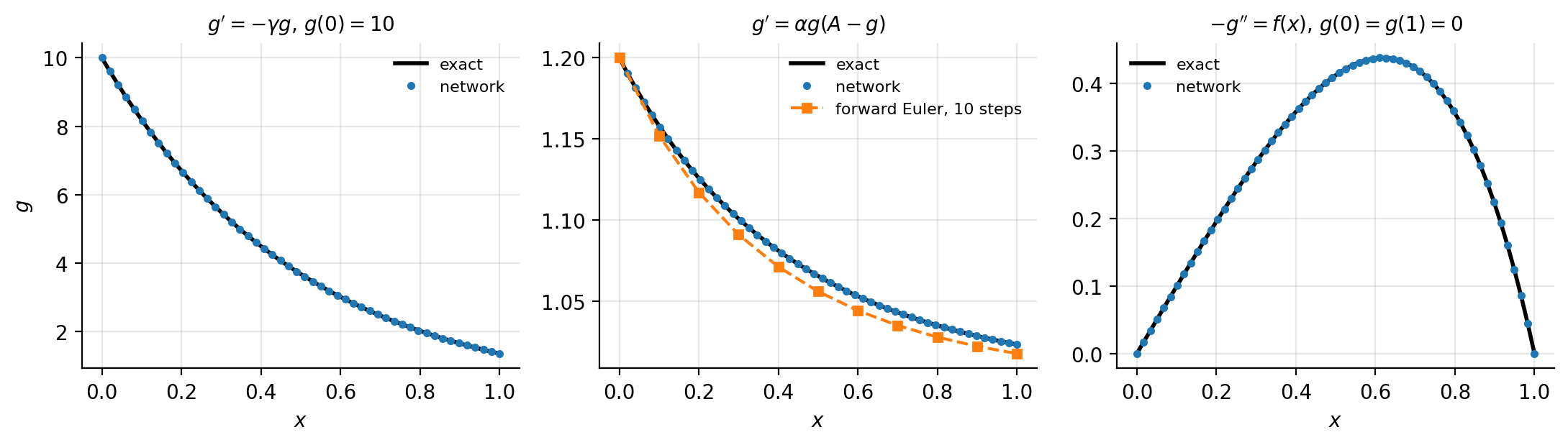
Figure 9.2: The three ordinary differential equations of Sections Exponential decay–The one-dimensional Poisson equation, with the network solution against the exact one. The middle panel adds the forward Euler solution with ten steps for comparison.
For a one-dimensional boundary-value problem on a simple domain, the classical method wins decisively, and it would be dishonest to present this example as a demonstration of anything else. Its value is as a verification: the network reproduces a known answer to five significant figures, which licenses its use where no classical method is convenient.
9.6. Partial differential equations#
A partial differential equation involves a function of several variables and may contain any combination of partial derivatives. In general, for a function \(g(x_1,\dots,x_N)\),
where \(f\) involves mixed derivatives up to order \(n\), and additional conditions are again needed for uniqueness.
The strategy is unchanged. We need a trial solution
in which \(h_1\) alone satisfies the conditions and \(h_2\) is built so that the network contributes nothing where they are imposed. The cost is again the mean squared residual, now over a set of \(M\) points \(\bm{x}_i=(x_1^{(i)},\dots,x_N^{(i)})\) forming the rows of a matrix \(\bm{X}\):
The only change to the network is that the input layer now has \(N\) nodes rather than one. Everything else – the architecture, the initialisation, the optimiser – is carried over from Chapter 8 unchanged, which is the point of having built it generally.
Partial derivatives in the code. For the ODEs we differentiated the network directly, using the recursions (9.5) and (9.6). For the PDEs the trial solutions become more elaborate, and hand-differentiating each one is error-prone drudgery of exactly the kind Section Automatic differentiation warned against. We therefore differentiate the trial solution itself, by nesting automatic differentiation with respect to one input coordinate at a time.
def d_dxk(fun, k):
    """Partial derivative of fun(P, X) with respect to input column k.

    Nesting this gives higher derivatives: d_dxk(d_dxk(u, 0), 0) is
    the second derivative with respect to x_0.
    """
    def wrapped(P, X):
        def scalarised(xk):
            Xn = np.concatenate([X[:, :k], xk.reshape(-1, 1), X[:, k+1:]], axis=1)
            return fun(P, Xn)
        return elementwise_grad(scalarised)(X[:, k])
    return wrapped
9.7. The diffusion equation#
In one spatial dimension the diffusion equation reads
and we impose
with \(u(x)=\sin(\pi x)\). For this initial condition the exact solution is
which decays rapidly – by a factor of \(e^{-\pi^{2}}\approx5\times10^{-5}\) over a unit of time.
The trial solution. Three conditions must hold: two boundaries in \(x\) and one initial condition in \(t\). The choice
satisfies all three identically. At \(t=0\) the second term vanishes and the first reduces to \(u(x)\); at \(x=0\) and \(x=1\) the factor \(x(1-x)\) kills the network while \(u(0)=u(1)=0\) kills the first term. Here \(h_1(x,t)=(1-t)u(x)\) and \(h_2=x(1-x)tN\).
nx, nt = 20, 20
xs, ts = np.linspace(0, 1, nx), np.linspace(0, 1, nt)
Xg, Tg = np.meshgrid(xs, ts, indexing="ij")
X = np.column_stack([Xg.ravel(), Tg.ravel()])       # M = 400 collocation points

def trial_diffusion(P, X):
    """Eq. (9.trialdiff)."""
    x, t = X[:, 0], X[:, 1]
    return (1 - t) * np.sin(np.pi * x) + x * (1 - x) * t * network(P, X, "tanh")

u_t  = d_dxk(trial_diffusion, 1)
u_x  = d_dxk(trial_diffusion, 0)
u_xx = d_dxk(u_x, 0)

def residual_diffusion(P, X):
    return u_t(P, X) - u_xx(P, X)                   # Eq. (9.diffusion)

P, history = solve_de(residual_diffusion, [2, 30, 30, 1], X, "tanh",
                      n_iter=800, gamma=1e-2, rng=np.random.default_rng(1))
After \(800\) iterations the maximum absolute error over the whole space-time grid is \(1.0\times10^{-2}\), and slicing by time,
t=0.000: max err 0.00e+00
t=0.105: max err 1.68e-03
t=0.316: max err 4.50e-04
The first line is the point of the construction. The error at \(t=0\) is exactly zero – not small, but zero to machine precision – because Eq. (9.29) satisfies the initial condition identically, whatever the parameters happen to be. No amount of training was required to achieve it and no amount of bad training could destroy it. The same is true along both spatial boundaries. A formulation that instead added the boundary conditions to the loss as extra terms would satisfy them only approximately, and would have to trade that accuracy against the interior residual.
The remaining error is concentrated at small but non-zero times, where the solution is changing fastest; by \(t=0.3\) the solution has decayed by a factor of twenty and the absolute error with it.
9.8. The wave equation#
The wave equation is second order in both variables,
with \(c\) the wave speed. The conditions are now four, since a second-order equation in time requires both the initial displacement and the initial velocity:
We take \(c=1\), \(u(x)=\sin(\pi x)\) and \(v(x)=0\), for which the exact solution is the standing wave
The trial solution. The extra condition on \(\partial g/\partial t\) at \(t=0\) requires a little more care, and the device is to use \(t^{2}\) rather than \(t\):
At \(t=0\) this gives \(u(x)\) as required. Differentiating with respect to \(t\) produces a factor \(t\) in every term – from \(-2t\,u(x)\) and from the product rule on \(t^{2}N\) – so the time derivative vanishes at \(t=0\), matching \(v(x)=0\). Both conditions hold identically for every \(P\). Had \(v\) been non-zero we would add a term \(t\,v(x)\), which contributes \(v(x)\) to the derivative at \(t=0\) and nothing to the value.
c = 1.0

def trial_wave(P, X):
    """Eq. (9.trialwave); the t^2 makes dg/dt vanish at t = 0."""
    x, t = X[:, 0], X[:, 1]
    return (1 - t**2) * np.sin(np.pi * x) + x * (1 - x) * t**2 * network(P, X, "tanh")

w_t, w_x = d_dxk(trial_wave, 1), d_dxk(trial_wave, 0)
w_tt, w_xx = d_dxk(w_t, 1), d_dxk(w_x, 0)

def residual_wave(P, X):
    return w_tt(P, X) - c**2 * w_xx(P, X)           # Eq. (9.wave)

P, history = solve_de(residual_wave, [2, 30, 30, 1], X, "tanh",
                      n_iter=800, gamma=1e-2, rng=np.random.default_rng(1))
The maximum absolute error over the grid is \(8.0\times10^{-3}\) after \(800\) iterations, on a solution of amplitude one. Note that this problem requires \(\partial^{2}/\partial t^{2}\) as well as \(\partial^{2}/\partial x^{2}\), so the smoothness argument of Section Differentiating the network with respect to its input applies in both variables: a piecewise-linear activation would give identically zero on both sides of Eq. (9.30) and would report a perfect residual of zero for a completely wrong solution. That failure mode – a satisfied residual and a meaningless answer – is worth keeping in mind whenever a residual falls suspiciously fast.
Figure 9.3 shows both partial differential equations. The left and right panels give time slices against the exact solutions; the middle panel gives the absolute error of the diffusion solution over the whole space-time domain. The error map is worth studying: it vanishes identically along all three edges where conditions were imposed – \(t=0\), \(x=0\) and \(x=1\) – which is the trial solution (9.29) doing its work, and it is largest at small non-zero times where the solution changes fastest.
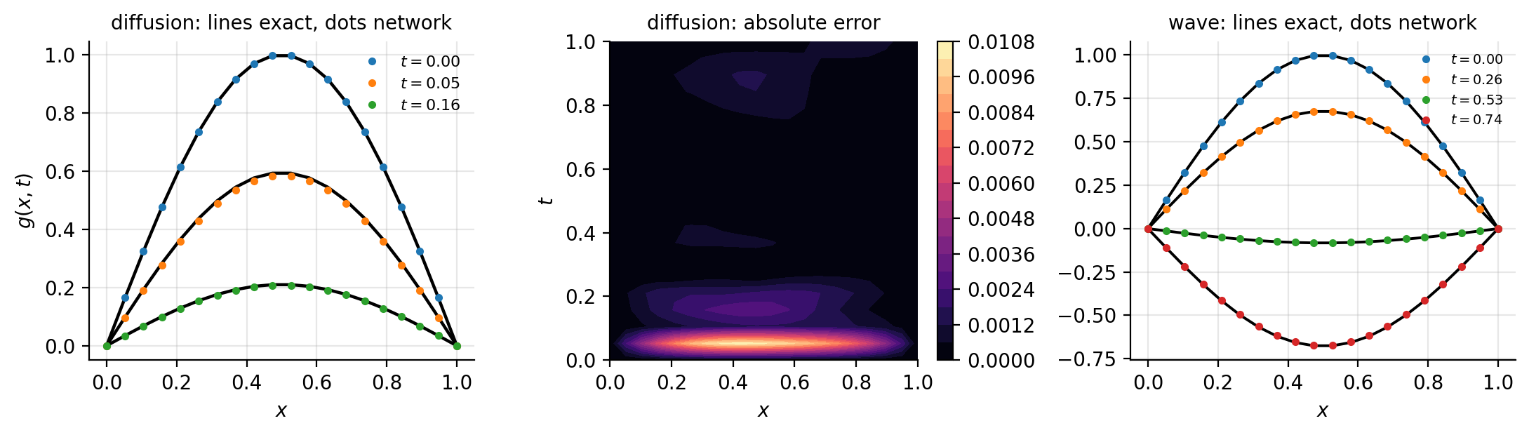
Figure 9.3: Left: time slices of the diffusion solution against the exact \(e^{-\pi^{2}t}\sin(\pi x)\). Centre: absolute error over the space-time domain, vanishing identically on the three edges where conditions are imposed. Right: time slices of the wave solution against \(\cos(\pi t)\sin(\pi x)\).
9.9. When is this worth doing?#
The comparisons above were deliberately unflattering. On the logistic equation a Runge-Kutta scheme is faster and more accurate; on the one-dimensional Poisson equation a tridiagonal solve is faster by orders of magnitude and just as accurate; on the diffusion equation an explicit finite-difference scheme would do very well. For textbook problems in one or two dimensions, classical numerical analysis wins, and it wins comfortably. Any presentation of this material that omits the comparison is selling something.
The case for the network method rests on the situations where classical methods become awkward.
High dimension. A finite-difference or finite-element method needs a mesh, and the number of mesh points grows exponentially with the number of dimensions. A network takes collocation points, which may be sampled randomly, and its cost grows with the number of parameters rather than with the volume of the domain. For equations in five or ten dimensions – the Hamilton-Jacobi-Bellman equation, the many-body Schr”odinger equation – meshes are impossible and networks are not.
Complicated geometry. Collocation points need no mesh, so an irregular domain costs nothing extra beyond sampling it.
The solution as a function. A finite-difference method returns values on a grid; interpolating between them is an extra step with its own error. The network returns a differentiable closed-form function valid everywhere in the domain, which can be evaluated, differentiated and composed at will.
Inverse problems and data assimilation. This is the strongest case. If some parameter of the equation is unknown but measurements of the solution are available, one simply adds a data-misfit term to Eq. (9.25) and optimises over the equation parameters alongside the network weights. The machinery is unchanged; for a classical solver this would require an adjoint calculation and a separate optimisation loop. This combination of equation and data is what the term physics-informed neural network usually refers to, and it is the subject we take up next.
Machine learning connection
The cost function (9.25) should be recognised as a regression problem in disguise, with the residual playing the role of the target and the collocation points the role of the data. Everything in Chapters 4 and 8 therefore applies without modification – and so do the difficulties. The optimisation is non-convex, as Section Exponential decay demonstrated painfully; the conditioning arguments of Section The learning rate and the condition number govern how quickly it converges; the choice of activation function decides whether the required derivatives exist at all; and there is no analogue of the convergence theory that tells us a finite-difference scheme is \(\bigO(\Delta x^{2})\). We have traded a method with guarantees for one with flexibility, and the exchange is worth making only when the flexibility is needed.
9.10. Physics-informed neural networks#
Everything so far has rested on the trial solution \(g_t=h_1+h_2(\bm{x},N)\). It is an elegant device and, as Section The diffusion equation showed, a powerful one: the conditions hold to machine precision for every value of the parameters, and the optimiser is left with the single job of satisfying the equation.
It is also a straitjacket. Constructing \(h_1\) and \(h_2\) requires a function that satisfies the conditions and a second function that vanishes wherever they are imposed, and both must be written down by hand for each new problem. For the box \([0,1]^{2}\) with homogeneous Dirichlet conditions this is easy, and \(x(1-x)\) does the job. For a domain that is not a box, for conditions imposed on a curved boundary, for a Neumann or Robin condition, or for a system of coupled equations, it ranges from tedious to impossible. The factor \(x(1-x)t\) in Eq. (9.29) has no counterpart on an L-shaped domain or an annulus.
The physics-informed neural network takes the opposite view. We drop the trial solution entirely and let the network itself be the approximate solution,
with no algebraic scaffolding whatsoever. Nothing then guarantees the boundary and initial conditions, so they are demanded of the optimiser instead: each condition contributes its own least-squares penalty to the cost. The conditions become soft constraints, satisfied approximately at the optimum, in place of the hard constraints of Eqs. (9.29) and (9.33), which held identically.
The material of this section follows a tutorial written for this course by Fredrik Nys{\ae}ter, Oskar Fausko and Kristian Liodden, transcribed into the framework built up in this chapter.
The composite cost function. Take the diffusion problem of Section The diffusion equation again. We need four sets of points rather than one. The collocation points \(\{(x_i,t_i)\}_{i=1}^{N_{\mathrm{pde}}}\) lie in the interior, where the equation is to hold; the initial points \(\{(x_i,0)\}\) lie on \(t=0\); and two sets of boundary points lie on \(x=0\) and \(x=1\). Each set gets a residual. For the equation itself,
which is exactly the cost (9.25) we have been minimising all along, only with \(N\) in place of \(g_t\). For the initial condition,
and for the two boundaries,
The quantity actually minimised is a weighted sum,
with positive weights \(\lambda\) whose choice we return to below.
Equation (9.38) should look familiar. It is a least-squares problem with several groups of targets, and the weights play the role of the penalty parameters of Section Ridge regression: they say how much we care about one group of residuals relative to another. Nothing in the machinery of Chapters 4 and 8 needs to change.
Implementation. The code is correspondingly small, because everything it needs already exists. The network is \verb!network! from Section Differentiating the network with respect to its input, the derivatives come from \verb!d_dxk! of Section Partial differential equations, the initialisation and the optimiser are those of Chapter 8. The only new element is that the cost sums several mean-squared residuals, each evaluated on its own set of points.
def pinn_solve(terms, layer_sizes, activation="tanh", n_iter=2000, gamma=1e-2,
               rng=None, every=200):
    """terms: list of (name, weight, residual_fn, points), Eq. (9.pinntotal).

    Each residual_fn(P, X) returns the residual on its own point set, so the
    equation, the initial condition and the boundaries are treated alike.
    """
    P = init_parameters(layer_sizes, activation, rng)

    def cost(P):
        total = 0.0
        for _, w, residual, Xk in terms:
            total = total + w * np.mean(residual(P, Xk) ** 2)
        return total

    return adam_minimise(cost, P, n_iter=n_iter, gamma=gamma)
Contrast this with \verb!solve_de!, which took a single residual on a single set of points. That is the whole difference between the two formulations at the level of code: one point set becomes several, and the cost acquires weights.
The diffusion equation revisited. We solve exactly the problem of Section The diffusion equation – Eq. (9.26) with the conditions (9.27) and \(u(x)=\sin\pi x\) – so that the two formulations can be compared on identical ground. The architecture is the same \([2,30,30,1]\) network with \(\tanh\) activation, and Adam with \(\gamma=10^{-2}\).
nx, nt = 20, 20
xs, ts = np.linspace(0, 1, nx), np.linspace(0, 1, nt)

Xi, Ti = np.meshgrid(xs[1:-1], ts[1:-1], indexing="ij")   # interior only
X_col = np.column_stack([Xi.ravel(), Ti.ravel()])         # 324 points
X_ic  = np.column_stack([xs, np.zeros(nx)])               # t = 0
X_l   = np.column_stack([np.zeros(nt), ts])               # x = 0
X_r   = np.column_stack([np.ones(nt),  ts])               # x = 1

def u_net(P, X): return network(P, X, "tanh")             # Eq. (9.pinnu)

u_t = d_dxk(u_net, 1)
u_x = d_dxk(u_net, 0)
u_xx = d_dxk(u_x, 0)

def r_pde(P, X): return u_t(P, X) - u_xx(P, X)            # Eq. (9.pinnpde)
def r_ic(P, X):  return u_net(P, X) - np.sin(np.pi * X[:, 0])
def r_bc(P, X):  return u_net(P, X)

terms = [("pde", 1.0, r_pde, X_col), ("ic",  10.0, r_ic, X_ic),
         ("bcL", 10.0, r_bc, X_l),   ("bcR", 10.0, r_bc, X_r)]

P, history = pinn_solve(terms, [2, 30, 30, 1], "tanh", n_iter=4000, gamma=1e-2,
                        rng=np.random.default_rng(1))
Note that the collocation points deliberately exclude the boundaries. A point that carries both the equation residual and a boundary residual is being asked two things at once, and the two requests compete.
The results, measured on a \(100\times100\) grid against the exact solution (9.28), are collected in Table 9.1, together with the hard-constraint results of Section The diffusion equation obtained with the same architecture and the same optimiser.
\noalign{} Formulation |
Iterations |
max error |
RMSE |
error at \(t=0\) |
|---|---|---|---|---|
\noalign{}\noalign{} Hard, Eq. (9.29) |
\(800\) |
\(1.04\times10^{-2}\) |
\(1.72\times10^{-3}\) |
\(0\) exactly |
Hard, Eq. (9.29) |
\(4000\) |
\(1.09\times10^{-2}\) |
\(1.66\times10^{-3}\) |
\(0\) exactly |
Soft, \(\lambda=1\) |
\(800\) |
\(2.62\times10^{-2}\) |
\(6.08\times10^{-3}\) |
\(2.62\times10^{-2}\) |
Soft, \(\lambda=10\) |
\(800\) |
\(2.98\times10^{-2}\) |
\(5.73\times10^{-3}\) |
\(1.36\times10^{-2}\) |
Soft, \(\lambda=100\) |
\(800\) |
\(3.00\times10^{-2}\) |
\(1.07\times10^{-2}\) |
\(3.00\times10^{-2}\) |
Soft, \(\lambda=10\) |
\(4000\) |
\(3.35\times10^{-2}\) |
\(6.77\times10^{-3}\) |
\(7.21\times10^{-3}\) |
\noalign{} |
Table 9.1: The diffusion equation solved two ways with the same network, optimiser and learning rate. The last column is the largest error on the line \(t=0\), where the initial condition is imposed.
The hard formulation wins, and it wins on every measure. Its root-mean-square error is three to four times smaller, and its error at \(t=0\) is not merely smaller but exactly zero, as it must be. Five times more training does not close the gap; the soft solution’s largest error is still \(3\times10^{-2}\) after \(4000\) iterations, and it sits at \(x=0.465\), \(t=0.040\), in the region where the solution is decaying fastest.
This is worth stating plainly, because presentations of physics-informed networks do not always state it: on a problem where a trial solution can be constructed, constructing it is better. Information built into the ansatz is free and exact; information supplied through the cost function must be paid for in optimisation effort and is never exact.
The weights are a real difficulty. Table 9.1 shows something else. Raising \(\lambda\) from \(1\) to \(10\) cuts the error at \(t=0\) roughly in half but leaves the overall error unchanged; raising it to \(100\) makes everything worse, because the optimiser now spends its capacity on the boundary at the expense of the equation, and \(L_{\mathrm{PDE}}\) rises by nearly an order of magnitude. There is a best \(\lambda\), it is problem-dependent, and we found it by trying three values.
The underlying reason is a conditioning problem of the kind discussed in Section The learning rate and the condition number. The four terms in (9.38) have gradients of very different magnitudes – \(L_{\mathrm{PDE}}\) involves a second derivative of the network and therefore carries factors of \(\bm{W}^{2}\), while \(L_{\mathrm{IC}}\) involves the network value alone – so the composite cost is far more anisotropic than any of its parts. A single learning rate must serve all of them. Figure 9.4(a) shows the consequence: the four terms fall at different rates and by different amounts, and they do not fall smoothly. Choosing the weights automatically, by balancing gradient magnitudes or by using the neural tangent kernel, is an active area of research and is not a solved problem.
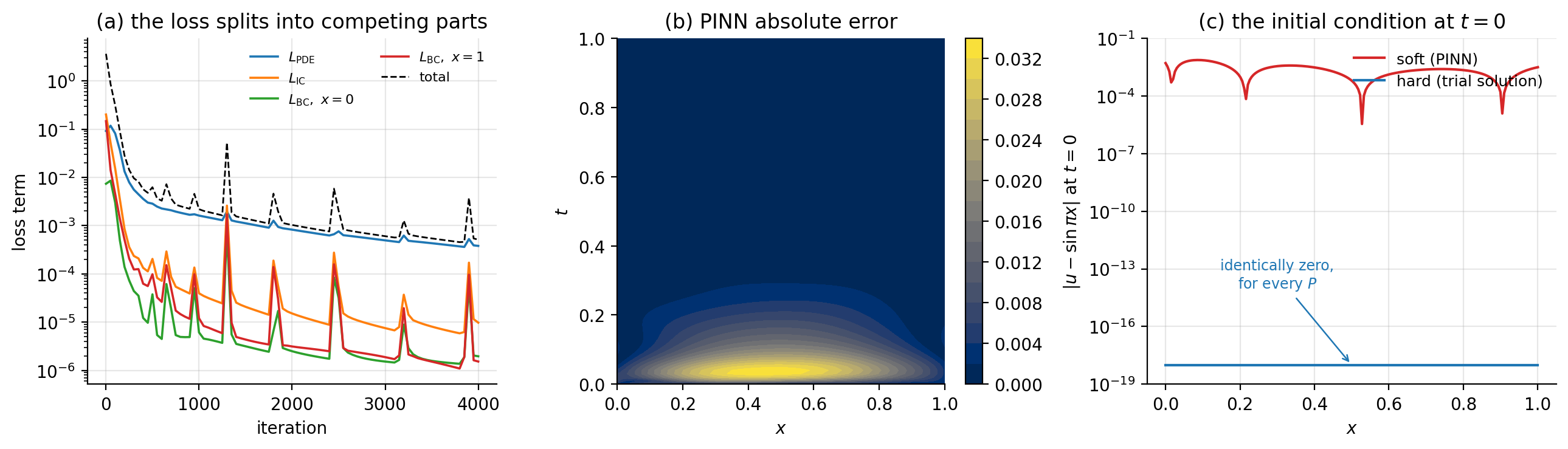
Figure 9.4: The diffusion equation solved with soft constraints. (a) The four terms of Eq. (9.38) during training, with \(\lambda=10\); they descend at different rates and the intermittent spikes are the terms trading against one another. (b) Absolute error of the converged solution, largest in the fast-decaying region near \(t=0\) rather than on the boundaries. (c) The initial condition at \(t=0\): the soft formulation misses it by up to \(7\times10^{-3}\), while the hard formulation of Section The diffusion equation satisfies it identically, for every value of the parameters.
Panel (c) of the figure makes the comparison as sharply as it can be made. The hard-constraint curve is not small; it is zero, and it would be zero for an untrained network. The soft-constraint curve is a genuine error that training reduces but never removes.
The wave equation revisited. Where the soft formulation pays off in convenience is the initial velocity. Recall the trouble it caused in Section The wave equation: to make \(\partial g_t/\partial t\) vanish at \(t=0\) we had to replace \(t\) by \(t^{2}\) throughout Eq. (9.33), and had \(v(x)\) been non-zero we would have needed a further term \(t\,v(x)\) whose interaction with the rest of the ansatz must be checked by hand. A condition on a derivative, imposed exactly, takes thought.
Imposed softly it takes one line, because a derivative residual is no different from any other residual:
def u_net(P, X): return network(P, X, "tanh")
u_t, u_x = d_dxk(u_net, 1), d_dxk(u_net, 0)
u_tt, u_xx = d_dxk(u_t, 1), d_dxk(u_x, 0)

def r_pde(P, X): return u_tt(P, X) - c**2 * u_xx(P, X)    # Eq. (9.wave)
def r_ic(P, X):  return u_net(P, X) - np.sin(np.pi * X[:, 0])
def r_iv(P, X):  return u_t(P, X)                    # dg/dt = v(x) = 0 at t=0
def r_bc(P, X):  return u_net(P, X)

terms = [("pde", 1.0, r_pde, X_col), ("ic", 10.0, r_ic, X_ic),
         ("iv",  10.0, r_iv,  X_ic),                 # the initial velocity
         ("bcL", 10.0, r_bc,  X_l), ("bcR", 10.0, r_bc, X_r)]

P, history = pinn_solve(terms, [2, 30, 30, 1], "tanh", n_iter=4000, gamma=1e-2,
                        rng=np.random.default_rng(1))
The line \verb!r_iv! is the entire treatment of the initial velocity. Changing \(v(x)\) from zero to anything else means editing that one line; no part of the construction has to be rethought. A Neumann boundary condition \(\partial u/\partial x=q\) would be added the same way, and so would a Robin condition \(\alpha u+\beta\,\partial u/\partial x=q\), neither of which fits comfortably into a trial solution.
The accuracy, however, tells the same story as before:
Soft, lambda=10,  800 it : max err 1.20e-02   rmse 4.44e-03
Soft, lambda=10, 4000 it : max err 8.73e-03   rmse 3.34e-03
Soft, lambda=50, 4000 it : max err 1.39e-02   rmse 4.99e-03
Hard, Eq. (9.trialwave),  800 it : max err 8.07e-03   rmse 2.21e-03
Hard, Eq. (9.trialwave), 4000 it : max err 4.81e-04   rmse 1.80e-04
The soft solution after \(4000\) iterations is about as good as the hard solution after \(800\), and the hard solution given the same \(4000\) iterations is eighteen times better. The gap here is wider than for the diffusion equation, and the reason is instructive: the standing wave \(\cos(\pi t)\sin(\pi x)\) has amplitude one throughout the domain, so the boundary terms never become negligible and continue to compete with the equation residual for the whole of training. In the diffusion problem the solution decays by a factor of \(2\times10^{4}\) and the competition fades.
So why use soft constraints at all?. Because of the last item in Section When is this worth doing?. Suppose the diffusion coefficient \(D\) in
is unknown, and instead we have a handful of noisy measurements \(\{(\bm{x}_i,y_i)\}\) of the solution at scattered points. This is an inverse problem, and for a classical solver it is a serious undertaking: one wraps the solver in an outer optimisation loop and differentiates through it, usually via an adjoint equation derived by hand for the problem at hand.
For a physics-informed network it is one more term in the cost and one more number in the parameter list. We minimise
over the weights and \(D\) together. Note what is not in Eq. (9.40): no initial condition and no boundary conditions. We are not told them; the data replace them. A trial solution cannot even be written down here, so the soft formulation is not merely more convenient, it is the only one available.
Since \(D\) is not a weight matrix, the optimiser must accept a slightly more general parameter object. Flattening is the tidy way to arrange this:
from autograd.misc import flatten

def adam_general(cost, params, n_iter=2000, gamma=1e-2, b1=0.9, b2=0.999, eps=1e-8):
    """Adam on any nested list of arrays -- here the weights and the scalar D."""
    flat, unflatten = flatten(params)
    gradient = grad(lambda f: cost(unflatten(f)))
    m = np.zeros_like(flat)
    v = np.zeros_like(flat)
    for it in range(1, n_iter + 1):
        g = gradient(flat)
        m = b1 * m + (1 - b1) * g
        v = b2 * v + (1 - b2) * g ** 2
        flat = flat - gamma * (m / (1 - b1**it)) / (np.sqrt(v / (1 - b2**it)) + eps)
    return unflatten(flat)
The problem itself is then four lines. We generate forty observations from the exact solution with \(D_{\mathrm{true}}=0.5\), corrupt them with Gaussian noise of standard deviation \(0.01\), and start the search from \(D_0=2.0\), four times too large.
D_true = 0.5
rng = np.random.default_rng(3)
X_obs = np.column_stack([rng.uniform(0, 1, 40), rng.uniform(0, 1, 40)])
y_obs = np.exp(-D_true * np.pi**2 * X_obs[:, 1]) * np.sin(np.pi * X_obs[:, 0]) \
        + rng.normal(0, 0.01, 40)

def u_net(P, X): return network(P[0], X, "tanh")     # P = [weights, D]
u_t, u_x = d_dxk(u_net, 1), d_dxk(u_net, 0)
u_xx = d_dxk(u_x, 0)

def cost(P):
    D = P[1][0]
    return np.mean((u_t(P, X_col) - D * u_xx(P, X_col)) ** 2) \
         + 10.0 * np.mean((u_net(P, X_obs) - y_obs) ** 2)   # Eq. (9.pinninv)

P = [init_parameters([2, 30, 30, 1], "tanh", np.random.default_rng(1)),
     np.array([2.0])]                                 # initial guess D_0 = 2
P = adam_general(cost, P, n_iter=3000, gamma=1e-2)
  it     1  cost 1.8735e+00  D 1.990000
  it   500  cost 2.5141e-02  D 1.673616
  it  1000  cost 7.0864e-03  D 0.637187
  it  1500  cost 2.7637e-03  D 0.496297
  it  2000  cost 2.3463e-03  D 0.512378
  it  2500  cost 1.4782e-03  D 0.507987
  it  3000  cost 1.3524e-03  D 0.515397

D_true = 0.5, recovered D = 0.515397, rel err 3.08%
Forty noisy points and no boundary information at all recover the coefficient to three per cent, and Figure 9.5(a) shows that starting values of \(D_0=2.0\), \(1.0\) and \(0.1\) all converge to the same answer. The network and the coefficient are found together, in one optimisation, by the same Adam update, and the only line of code that knows this is an inverse problem is \verb!D = P[1][0]!.
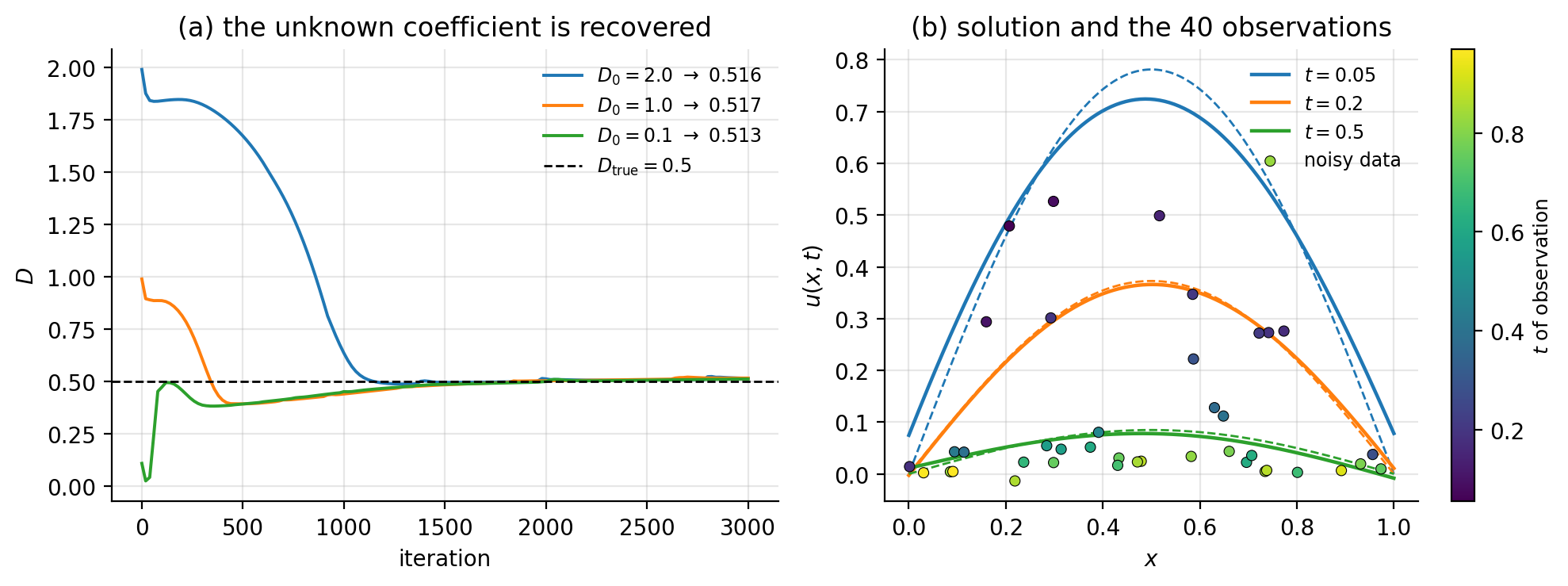
Figure 9.5: Recovering an unknown diffusion coefficient from forty noisy observations. (a) The estimate of \(D\) during training from three different starting values, converging to \(D\approx0.515\) against a true value of \(0.5\). (b) The recovered solution at three times, solid, against the exact solution, dashed, with the observations shaded by the time at which they were taken. The visible gap at \(t=0.05\) is the three per cent error in \(D\).
The result should not be oversold. Inverse problems are ill-posed, and the recovered coefficient degrades quickly as the data get noisier:
noise   D_recovered   rel.err
 0.00   0.4770         4.59%
 0.01   0.5154         3.08%
 0.05   0.6888        37.76%
The first two rows differ by less than the scatter between random seeds and should be read as the same result. The third should not: five per cent noise on the observations produces a thirty-eight per cent error in \(D\). The sensitivity is a property of the inverse problem and not of the method – a classical adjoint-based inversion on the same data would face it too – but it is a reminder that recovering parameters from data is a statistical estimation problem, with all that Chapter 2 implies about variance and about the danger of reporting a single number without an error estimate.
Soft or hard?. The two formulations are not rivals so much as two points on a scale, and the question is how much of what we know can be built into the ansatz rather than requested through the cost.
If a trial solution can be constructed, construct it. The conditions then hold exactly, the cost has one term, there are no weights to tune, and Table 9.1 shows the accuracy that buys.
If the geometry is awkward, the conditions involve derivatives or mixed terms, or the equations are coupled, use soft constraints. The loss of accuracy is real but bounded, and the alternative may be no method at all.
If parameters of the equation are unknown and data are available, soft constraints are the only option, and they are extremely convenient.
Nothing prevents mixing the two. A trial solution can enforce the boundary conditions exactly while an initial condition is handled by a penalty, and this hybrid is often the best of the three.
A last practical remark, and it applies to both formulations. Both networks above were trained on a \(20\times20\) grid of points and evaluated on a \(100\times100\) grid; the errors quoted throughout are the evaluation-grid errors. This is not interpolation in the finite-difference sense but simple evaluation of a closed-form function, and it is one thing the method genuinely does better than a grid-based scheme, which returns numbers at grid points and nothing in between.
9.11. A stochastic equation: Black-Scholes option pricing#
Every equation solved so far was deterministic and had homogeneous boundary conditions on a unit box. The Black-Scholes equation of mathematical finance has neither property, and it arrives by a different route: it is the deterministic equation satisfied by the price of a derivative whose underlying asset follows a stochastic process. It therefore makes a good final test, and it is the problem for which the physics-informed formulation of Section Physics-informed neural networks is not a convenience but a necessity.
9.11.1. From a stochastic process to a deterministic equation#
Assume the price \(S_t\) of an asset follows geometric Brownian motion,
where \(\mu\) is the drift, \(\sigma>0\) the volatility and \(W_t\) a Wiener process, so that \(\mathrm{d}W_t\) is normally distributed with mean zero and variance \(\mathrm{d}t\). The multiplicative form matters: it keeps \(S_t>0\) and makes the relative return \(\mathrm{d}S_t/S_t\) the quantity with stationary statistics, which is what the empirical distributions of Chapter 2 suggest for asset prices.
Let \(C(S,t)\) be the price of a derivative written on this asset. Because \(S_t\) is a stochastic process, ordinary calculus does not apply to \(C(S_t,t)\); the correct chain rule is It^o’s lemma, which for a twice-differentiable \(C\) reads
The extra second-derivative term, absent from the deterministic chain rule, is the whole content of It^o calculus: it appears because \((\mathrm{d}W_t)^{2}=\mathrm{d}t\) rather than \(\bigO(\mathrm{d}t^{2})\), so the second-order term in a Taylor expansion survives the limit.
Now form the portfolio \(\Pi = C - \Delta\,S\) consisting of one derivative and a short position of \(\Delta\) units of the asset. Using Eqs. (9.41) and (9.42),
The choice
annihilates the second bracket, and with it the \(\mathrm{d}W_t\) term. The portfolio has become riskless over the infinitesimal interval, and a riskless portfolio must earn the risk-free rate \(r\) on pain of arbitrage, \(\mathrm{d}\Pi = r\Pi\,\mathrm{d}t\). Equating the two expressions and dividing by \(\mathrm{d}t\) gives the Black-Scholes equation,
on \(S>0\), \(0\le t\le T\).
Two features of this derivation are worth recording. The drift \(\mu\) has disappeared: the price of the derivative does not depend on how fast the underlying is expected to grow, only on how much it fluctuates. And the equation is deterministic even though its subject is stochastic – the randomness has been hedged away by Eq. (9.44), and what remains is a partial differential equation of exactly the kind this chapter has been solving.
9.11.2. Conditions, and the link to the diffusion equation#
The contract is specified by conditions at maturity rather than at the start. For a European call option – the right, but not the obligation, to buy one unit of the asset at the strike price \(K\) at time \(T\) – the holder exercises only if \(S>K\), so
This is a terminal condition, and Eq. (9.45) is a backward parabolic equation: it is well posed running backwards from \(t=T\), exactly as the diffusion equation is well posed running forwards from \(t=0\). The substitution \(\tau=T-t\) turns one into the other and is the first thing to do in any implementation.
The boundary conditions in \(S\) follow from arbitrage arguments. If the asset becomes worthless it stays worthless, by Eq. (9.41), so the option expires unexercised:
If instead \(S\) is very large the option will certainly be exercised, and holding it is equivalent to holding the asset less the discounted strike:
In practice the domain is truncated at some \(S_{\max}\gg K\) and Eq. (9.48) imposed there.
This is the diffusion equation in disguise
Set \(x=\ln(S/K)\), \(\tau=\tfrac12\sigma^{2}(T-t)\) and \(u(x,\tau)=e^{\alpha x+\beta\tau}C(S,t)\). The chain rule gives \(\partial u/\partial x = e^{\alpha x+\beta\tau}(\alpha C + SC_S)\) and \(\partial^{2}u/\partial x^{2} = e^{\alpha x+\beta\tau} (\alpha^{2}C+(2\alpha+1)SC_S+S^{2}C_{SS})\), and the choices
reduce Eq. (9.45) to \(u_\tau = \tfrac12\sigma^{2}u_{xx}\), which is Eq. (9.26) up to the constant. The logarithm is what removes the variable coefficients \(S\) and \(S^{2}\); geometric Brownian motion is ordinary Brownian motion in \(\log S\). We do not exploit this in the solver below, and deliberately so: the transformation exists for this equation and not for the multi-asset or stochastic-volatility generalisations, whereas the network formulation is indifferent.
Because a closed form is available for this one-dimensional case, we can check the answer. The Black-Scholes formula is
with \(N\) the standard normal cumulative distribution and
9.11.3. Why a trial solution will not do#
Every construction of Sections The diffusion equation and The wave equation rested on finding \(h_1\) satisfying the conditions and \(h_2\) vanishing where they are imposed. Here that programme fails at the first step. The condition at the far boundary, Eq. (9.48), is inhomogeneous and time-dependent; the terminal condition (9.46) is not differentiable at \(S=K\); and the domain is a truncation of a half-line rather than a box. One can, with effort, manufacture an \(h_1\) that interpolates the three conditions, but it will be elaborate, problem-specific, and worthless the moment a second asset or a non-constant volatility is introduced.
The soft formulation asks for none of it. Each condition becomes a residual, exactly as in Eq. (9.38):
with \(L_{\mathrm{PDE}}\) the mean square of Eq. (9.45) at interior collocation points and the other three the mean squares of the misfits in Eqs. (9.46), (9.47) and (9.48).
9.11.4. Scaling matters more than anything else#
Before any code, a remark that turns out to dominate the result. In the variables of Eq. (9.45) the network is asked to take inputs \(S\in[0,20]\) and \(t\in[0,1]\) and produce outputs in \([0,15]\). A \(\tanh\) network initialised by Eq. (8.49) produces outputs of order one from inputs of order one; feeding it \(S=20\) saturates the first layer immediately. Worse, the residual (9.45) contains \(S^{2}C_{SS}\), whose magnitude varies by a factor of \(400\) across the domain, so the collocation points near \(S_{\max}\) dominate \(L_{\mathrm{PDE}}\) and the region near the strike – the only region anyone cares about – is effectively ignored.
The remedy is to non-dimensionalise. Measure the asset price in units of the strike and the option price likewise, and run time backwards:
under which Eq. (9.45) becomes
with terminal condition \(c(s,0)=\max(s-1,0)\) now an initial condition. The equation is unchanged in form – it is homogeneous of degree one in the price, which is why the strike is the natural unit – but the inputs and outputs are now of order one.
Table 9.2 shows what this is worth. Both runs use the same network, the same optimiser, the same weights, the same number of iterations and the same seed; they differ only in the choice of variables.
\noalign{} Variables |
max error |
RMSE |
final \(L_{\mathrm{PDE}}\) |
|---|---|---|---|
\noalign{}\noalign{} \((S,t)\) as written, Eq. (9.45) |
\(0.498\) |
\(0.272\) |
\(2.32\times10^{-2}\) |
\((s,\tau)\) scaled, Eq. (9.53) |
\(\mathbf{0.318}\) |
\(\mathbf{0.042}\) |
\(\mathbf{1.59\times10^{-4}}\) |
\noalign{} |
Table 9.2: The Black-Scholes equation with \(K=5\), \(T=1\), \(r=0.05\), \(\sigma=0.3\) and \(S_{\max}=20\), solved by a \([2,40,40,1]\) network with \(\tanh\) activation, Adam with \(\gamma=5\times10^{-3}\), \(\lambda=10\) and \(4000\) iterations. Errors are in units of the option price and measured on a \(120\times120\) grid against Eq. (9.49); the largest option value on the grid is about \(15\).
Non-dimensionalising improves the root-mean-square error by a factor of \(6.5\) and the equation residual by a factor of \(145\), at no computational cost whatsoever. This is the single most useful practical fact in the chapter, and it generalises: before training a physics-informed network on any problem with dimensional quantities, rescale so that inputs, outputs and each term of the residual are of order one.
9.11.5. Implementation#
The code is the machinery of Section Physics-informed neural networks with a different residual.
K, T, r, sigma, S_max = 5.0, 1.0, 0.05, 0.3, 20.0
hi = S_max / K                                  # domain in scaled units

def c_net(P, X): return network(P, X, "tanh")   # X = (s, tau)

c_tau = d_dxk(c_net, 1)
c_s = d_dxk(c_net, 0)
c_ss = d_dxk(c_s, 0)

def r_pde(P, X):                                # Eq. (9.bsscaledpde)
    s = X[:, 0]
    return (-c_tau(P, X) + 0.5 * sigma**2 * s**2 * c_ss(P, X)
            + r * s * c_s(P, X) - r * c_net(P, X))

def r_term(P, X):                               # payoff at tau = 0
    return c_net(P, X) - np.maximum(X[:, 0] - 1.0, 0.0)

def r_lo(P, X):                                 # c(0, tau) = 0
    return c_net(P, X)

def r_hi(P, X):                                 # c(hi, tau) = hi - exp(-r tau)
    return c_net(P, X) - (hi - np.exp(-r * X[:, 1]))

terms = [("pde", 1.0, r_pde, X_col), ("term", 10.0, r_term, X_term),
         ("lo", 10.0, r_lo, X_lo),   ("hi", 10.0, r_hi, X_hi)]

P, history = pinn_solve(terms, [2, 40, 40, 1], "tanh", n_iter=4000, gamma=5e-3,
                        rng=np.random.default_rng(1))
Nothing here is specific to finance beyond the four residuals. Replacing \verb!r_pde! by a two-asset Black-Scholes equation with a correlation term, or \verb!r_term! by the payoff of a different contract, is a one-line change in each case, and neither requires rethinking the construction.
9.11.6. Results#
The prices at \(t=0\), which is what a trader would actually want, come out as
   S   network    exact   abs err
  2.0    0.0050   0.0005   0.0044
  4.0    0.2437   0.2277   0.0160
  5.0    0.7301   0.7116   0.0186
  6.0    1.4423   1.4440   0.0017
  8.0    3.2608   3.2748   0.0139
 12.0    7.2684   7.2445   0.0239
so that an option worth \(\$0.71\) at the money is priced to about two cents, and one worth \(\$7.24\) deep in the money to about two cents as well. Whether that is good enough depends entirely on the application, and it is an order of magnitude worse than the closed form, which is exact.
More interesting is where the error lives. The largest discrepancy over the whole domain is \(0.318\), and it occurs at
max err 0.3179 at S=5.04 t=1.000  (K=5.0 T=1.0)
err  t>0.9 (near maturity): 0.3179    t<0.5: 0.1065
err  |S-K|<1 (near strike): 0.3179    |S-K|>3: 0.1458
that is, at \(S=K\) and \(t=T\) to within one grid spacing – precisely the corner where the payoff (9.46) has its kink. This is not an accident of training and it will not go away with more iterations. The exact solution is continuous but not differentiable there, while a \(\tanh\) network is infinitely differentiable everywhere; the network is being asked to represent a function it structurally cannot represent, and it does the best a smooth function can do, which is to round the corner off. Away from the kink, at \(t<0.5\) or more than three strikes from the money, the error falls by a factor of two to three. Figure 9.6(b) shows the whole error surface and the point where it peaks.
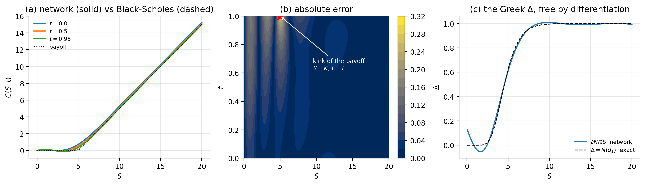
Figure 9.6: Black-Scholes by a physics-informed network. (a) The option price at three times, network solid and Eq. (9.49) dashed, with the terminal payoff (9.46) dotted; the vertical line is the strike. (b) Absolute error over the whole domain, peaking at the starred point \(S=K\), \(t=T\) where the payoff has its kink and the exact solution is not differentiable. (c) The hedge ratio \(\Delta=\partial C/\partial S\) obtained by differentiating the trained network, against the exact \(N(d_1)\). The network reproduces it without having been asked to, but goes slightly negative near \(S=2\), which no true option price can do.
The Greeks come for free. A practitioner needs not only the price but its sensitivities, of which the most important is the hedge ratio \(\Delta=\partial C/\partial S\) that appeared in Eq. (9.44). A finite-difference or lattice solver returns prices on a grid and \(\Delta\) must be recovered by numerical differentiation, which amplifies the error. The network is a differentiable closed-form function, so \(\Delta\) is one call to \verb!d_dxk!:
   S   network    exact   abs err
  2.0   -0.0441   0.0031   0.0472
  4.0    0.3553   0.3346   0.0206
  5.0    0.6103   0.6243   0.0139
  6.0    0.8012   0.8224   0.0212
  8.0    0.9795   0.9702   0.0094
 12.0    0.9965   0.9994   0.0029
Against \(\Delta=N(d_1)\) this is accurate to about two per cent over the range that matters, and the network was never trained on \(\Delta\) at all. It was trained on Eq. (9.45), and the derivative it produces is a consequence. This is the concrete form of the “solution as a function” argument of Section When is this worth doing?.
An honest failure. The first line of that table should not be passed over. At \(S=2\), deep out of the money, the network reports \(\Delta=-0.044\). A negative delta on a call option is impossible: the price of a call is non-decreasing in the price of the underlying, since a call on a more valuable asset cannot be worth less. The network has produced a small violation of a structural property that the exact solution satisfies identically, in a region where the option is nearly worthless and the residual is correspondingly insensitive. Figure 9.6(c) shows the dip.
This is worth generalising. The soft formulation enforces the equation and the conditions only in the mean-square sense, and nothing else at all. Monotonicity, convexity in \(S\), the no-arbitrage bounds \(\max(S-Ke^{-r(T-t)},0)\le C\le S\) – none of these is in the loss, so none is guaranteed, and a small residual is perfectly compatible with violating them where the solution is flat. A finite-difference scheme on this problem can be shown to preserve monotonicity under a step-size condition. We have traded a method with structural guarantees for one with flexibility, and this is what that trade costs. If such properties matter, they must be added to the loss as further penalty terms, or enforced by construction.
Why bother, if there is a closed form?
For a European call on a single asset there is no case for a network: Eq. (9.49) is exact and evaluates in microseconds. The case begins where the closed form ends. A basket option on \(d\) correlated assets satisfies a \(d\)-dimensional analogue of Eq. (9.45) with a full covariance matrix in the second-derivative term, for which no closed form exists and a finite-difference grid needs \(n^{d}\) points; at \(d=5\) this is already hopeless and the collocation approach of Section Partial differential equations is not. American options, which may be exercised early, turn the equation into a free boundary problem. Stochastic volatility replaces the constant \(\sigma\) by a second stochastic process and adds a dimension. And calibration – inferring the volatility surface from quoted market prices – is precisely the inverse problem of Section Physics-informed neural networks, with \(\sigma\) in place of \(D\). The one-dimensional call is the test case, not the application.
9.12. Summary and the programs#
This chapter used the network of Chapter 8 unchanged and asked it a different question. There were no labels; the differential equation supplied the only information, through the residual, and minimising the mean squared residual (9.3) was the training.
Three constructions carry the method. The trial solution \(g_t=h_1+h_2(x,N)\) builds the boundary and initial conditions into the ansatz so that they hold identically, for every value of the parameters – which is why the error of the diffusion solution at \(t=0\) was exactly zero rather than merely small. The optimiser is then asked to satisfy the equation and nothing else. And the forward-mode recursions (9.5) and (9.6) supply the derivatives of the network with respect to its input, propagating alongside the ordinary forward pass at a cost of one extra matrix product per layer per order. The third is the composite cost (9.38) of the physics-informed network, which abandons the trial solution and asks the optimiser for the conditions instead. Where both formulations apply, the trial solution is more accurate by a factor of three to eighteen at equal cost; the composite cost earns its place where no trial solution can be written down.
That second construction made concrete a claim left hanging in Chapter 8. Equation (9.6) requires \(f''\), and for ReLU and leaky ReLU this vanishes identically: the measured \(\max|\partial^{2}N/\partial x^{2}|\) was exactly \(0\) for both, against \(10^{-2}\) to \(1\) for every smooth activation. A rectified network cannot solve a second-order equation, and worse, it will report a residual of zero while doing so.
Six problems were solved and every one checked against its exact solution: exponential decay, logistic growth, the one-dimensional Poisson equation, the diffusion and wave equations – the last two in both the hard and the soft formulation – and the Black-Scholes equation of option pricing. Two were also compared against classical schemes, and the comparison was not flattering. Forward Euler and the three-point finite-difference formula are faster by orders of magnitude and comparably accurate; the network’s case rests instead on high dimension, irregular geometry, a differentiable closed-form solution, and above all on inverse problems, where data and equation can be combined in a single cost. Section Physics-informed neural networks made that last case concrete by recovering an unknown diffusion coefficient, \(D=0.515\) against a true \(0.5\), from forty noisy observations and no boundary information at all – a calculation for which the trial-solution formulation has nothing to offer, since there is no condition to build in.
Section A stochastic equation: Black-Scholes option pricing added the other half of the argument. The Black-Scholes equation (9.45) is the deterministic equation left behind when the randomness of geometric Brownian motion is hedged away, and its conditions – inhomogeneous, time-dependent, imposed at maturity rather than at the start, and non-differentiable at the strike – defeat the trial-solution construction entirely. Three lessons came out of it. Non-dimensionalising the problem, Eq. (9.52), improved the root-mean-square error by a factor of \(6.5\) and the residual by a factor of \(145\) for no cost at all, and is the first thing to try on any dimensional problem. The largest error sat exactly at the kink of the payoff, at \(S=K\) and \(t=T\), because a smooth network cannot represent a corner. And the hedge ratio \(\Delta=\partial C/\partial S\) came out to two per cent by differentiating a network that was never trained on it – against which must be set the fact that the same network reported a negative \(\Delta\) deep out of the money, violating a no-arbitrage property that nothing in the loss had asked it to respect.
The failure recorded in Section Exponential decay deserves to be remembered. A network of the wrong width settled into a local minimum at cost \(31.9\) and stayed there for ten thousand iterations, returning a solution wrong by eighteen per cent with no indication that anything was amiss. Non-convexity is not an abstraction, and a method that can converge confidently to the wrong answer must always be checked against something.
The programs are collected in the directory
doc/BookML/BookPrograms/chapter09_differential_equations.
Every listing printed above appears there as a numbered file, extracted automatically and in chapter order, and three of them are also provided as self-contained modules that run start to finish and reproduce the numbers quoted in the text:
nn_de.py– the network of Chapter 8 extended with the input-derivative recursions of Section Differentiating the network with respect to its input, the Adam minimiser andsolve_de. Everything else imports from here.pinn.py–pinn_solve, the composite cost (9.38), and the diffusion and wave equations in the soft formulation. Running it reproduces the soft-constraint rows of Table 9.1 and the wave-equation errors of Section Physics-informed neural networks.pinn_inverse.py–adam_generaland the recovery of the unknown diffusion coefficient from noisy data, together with the noise study.blackscholes.py– the Black-Scholes residuals of Section Implementation, the scaled and unscaled runs of Table 9.2, the price and \(\Delta\) tables, and the comparison against the closed form (9.49).
The figures are generated by the three scripts ch09_figures.py,
ch09_pinn_figures_a.py and ch09_pinn_figures_b.py in
doc/BookML/BookFigures; none is drawn by hand.
9.13. Exercises#
9.13.1. Warm-up exercises#
Trial solutions. Construct a trial solution of the form (9.2) for each of the following, and verify that the conditions hold identically: (a) \(g(0)=a\) and \(g(1)=b\) on \([0,1]\); (b) \(g(0)=a\) and \(g'(0)=v\); (c) \(g\) periodic on \([0,1]\), that is \(g(0)=g(1)\) and \(g'(0)=g'(1)\).
The derivative recursions. (a) Derive Eq. (9.5) from the forward pass (9.4). (b) Derive Eq. (9.6), being explicit about where the product rule is used. (c) Show that for a linear output layer no \(f'\) appears in the last step. (d) Count the operations and confirm that \(N\), \(N'\) and \(N''\) together cost about three forward passes.
Why ReLU fails. (a) Show that \(\mathrm{ReLU}''\equiv0\) wherever it is defined and hence that Eq. (9.6) gives zero throughout. (b) Confirm this numerically for a randomly initialised network. (c) Solve the Poisson problem of Section The one-dimensional Poisson equation with a ReLU network and report both the final residual and the actual error. Explain the discrepancy. (d) Repeat with GELU, Swish and \(\tanh\) and compare.
Exponential decay by hand. For the trial solution (9.9), write out the residual for a network with a single hidden unit, \(N(x)=w_2\tanh(w_1x+b_1)+b_2\), and obtain \(\partial C/\partial w_2\) analytically. Verify against automatic differentiation.
Collocation points (numerical). For the Poisson problem, vary the number of collocation points from \(10\) to \(200\). (a) Plot the final error against the number of points. (b) Compare with the \(\bigO(\Delta x^{2})\) behaviour of finite differences. (c) Try randomly sampled rather than uniformly spaced points, and comment.
Reproducing the local minimum. Reproduce the failure described in Section Exponential decay: two hidden layers of twenty units, \(\gamma=10^{-2}\). (a) Confirm that the cost stalls near \(31.9\) and does not move. (b) Plot the solution it returns against the exact one. (c) Find the smallest change – in width, learning rate or seed – that escapes it. (d) What diagnostic would have revealed the failure without knowing the exact solution?
Activation functions (numerical). Solve the diffusion equation with \(\tanh\), GELU, Swish, sigmoid and softplus, five seeds each. Report the median error and the spread, and compare your conclusions with Table 8.2 of Chapter 8.
A harder initial condition. Solve the diffusion equation with \(u(x)=\sin(\pi x)+\tfrac12\sin(3\pi x)\), whose exact solution superposes two modes decaying at different rates. (a) Verify against the exact solution. (b) Which mode is captured less well, and why?
Non-zero initial velocity. Modify the wave-equation trial solution (9.33) to accommodate \(v(x)\ne0\), as suggested in Section The wave equation. Verify that both conditions hold identically, then solve with \(v(x)=\sin(2\pi x)\) and check against the exact solution obtained by separation of variables.
Comparison with classical methods. For the diffusion equation, implement an explicit finite-difference scheme and compare against the network in accuracy, runtime and memory as the grid is refined. At what point, if any, does the network become competitive? Then repeat the argument in your head for a five-dimensional domain and explain why the answer changes.
9.13.2. Project-style exercise: a differential-equation solver#
Part a: the machinery. Implement the input-derivative recursions of Section Differentiating the network with respect to its input on top of your Chapter 8 network, and verify them against automatic differentiation to machine precision for every activation function. Produce the second-derivative table and confirm that the rectified family gives exactly zero.
Part b: ordinary equations. Solve the three ODEs of Sections Exponential decay to The one-dimensional Poisson equation, checking each against its exact solution. For each, compare against a classical scheme of your choice at matched cost, and present the comparison honestly.
Part c: robustness. For each problem, run ten seeds and report the median and spread of the error. Study the dependence on width, depth, learning rate and number of iterations. Identify at least one configuration that fails, and diagnose it.
Part d: partial equations. Solve the diffusion and wave equations with trial solutions. Plot the solution as a surface and as time slices against the exact solution, and verify that the conditions built into the trial solution hold to machine precision throughout training – not merely at the end.
Part e: a problem without an exact solution. Solve a problem for which no closed form is available – a non-linear Poisson equation, or diffusion with a spatially varying coefficient. Since you cannot check against the truth, design your own verification: mesh refinement of a classical solver, the residual on points not used for training, and consistency across seeds. Discuss what would convince you that the answer is right.
Part f: soft constraints. Re-solve both partial differential equations of part d with the composite cost (9.38) instead of a trial solution, and reproduce Table 9.1 for your own implementation. Scan \(\lambda\in\{1,10,100,1000\}\) and plot the four loss terms separately against the iteration count, as in Figure 9.4(a). Then answer two questions with evidence. Does the best \(\lambda\) for the diffusion equation remain the best for the wave equation? And is the error at \(t=0\) ever driven below the interior error, or does the initial condition remain the worst-satisfied part of the problem however \(\lambda\) is chosen?
Part g: an inverse problem. Take the diffusion equation with an unknown coefficient \(D\), generate synthetic noisy measurements at scattered points, and recover \(D\) as in Section Physics-informed neural networks. Go beyond the worked example in three directions. Study how the recovered \(D\) degrades as the measurements become sparser as well as noisier, and map the region of the (noise, \(N_{\mathrm{data}}\)) plane in which the answer is usable. Attach an uncertainty to \(D\) by bootstrapping the observations, using the machinery of Chapter 2, and report an interval rather than a number. Finally, make the coefficient a function \(D(x)\) rather than a constant – represent it by a second small network – and investigate at what point the problem becomes too ill-posed to solve.
Part h: option pricing. Reproduce Section A stochastic equation: Black-Scholes option pricing. (a) Derive Eq. (9.45) from Eqs. (9.41) and (9.42), and say precisely where the drift \(\mu\) cancels and why that is remarkable. (b) Verify the change of variables in the notebox of Section Conditions, and the link to the diffusion equation by carrying out the chain rule and solving for \(\alpha\) and \(\beta\). (c) Solve the equation with the composite cost and reproduce Table 9.2, confirming for yourself how much the scaling is worth. (d) Locate the largest error and confirm that it sits at the kink of the payoff. Then replace the call payoff by a smooth approximation, for instance \(\tfrac12\left(S-K+\sqrt{(S-K)^{2}+\epsilon^{2}}\right)\), and study how the error at the corner behaves as \(\epsilon\to0\). (e) Compute \(\Delta\), \(\Gamma=\partial^{2}C/\partial S^{2}\) and \(\mathcal{V}=\partial C/\partial\sigma\) from the trained network. The last one requires thought: \(\sigma\) is not an input, so either retrain over a range of \(\sigma\) with volatility as a third input, or use a finite difference in \(\sigma\) over two trainings. Compare against the closed-form Greeks. (f) Check the no-arbitrage bounds \(\max(S-Ke^{-r(T-t)},0)\le C\le S\) and the monotonicity and convexity of \(C\) in \(S\) over the whole grid, and report where your solution violates them. Then add a penalty term that punishes \(\min(\partial C/\partial S,0)\) and report whether it helps and what it costs elsewhere. (g) Extend to two correlated assets, for which
with the payoff \(\max(\max(S_1,S_2)-K,0)\). There is no closed form, so verify against a Monte Carlo estimate using Eq. (9.41) and the machinery of Chapter 2, and state how many paths you need for the Monte Carlo error to fall below the network error.
Part i: a domain that is not a box. Solve the Poisson equation \(-\nabla^{2}u=f\) on an L-shaped domain, or on an annulus, with \(u=0\) on the boundary. Sample collocation points in the interior and boundary points on the edges. Explain, in writing, why the trial-solution approach of Section The one-dimensional Poisson equation cannot be used here, and what that implies about the trade-off set out at the end of Section Physics-informed neural networks.