
10. Chapter 10: Convolutional Neural Networks#
The network of Chapter 8 treats its input as a vector. Whatever the data were before – an image, a sound clip, a spectrum – they are flattened into \(\bm{x}\in\mathbb{R}^{d}\) and multiplied by a dense weight matrix. Every input coordinate is treated identically and interchangeably: permute the pixels of every image in the training set by one fixed permutation and the network learns exactly as well, because nothing in an affine map knows that pixel \((i,j)\) sits next to pixel \((i,j+1)\).
For data with spatial or temporal structure this is throwing away information before training begins. Images, sound and volumetric scans share three properties that a vector does not record. They are stored as multi-dimensional arrays; they have one or more axes along which ordering matters; and they have a channel axis giving different views of the same location, such as the red, green and blue values of a pixel.
The convolutional neural network is the architecture obtained by insisting that the linear map respect this structure. This chapter builds it from the definition of convolution, establishes the properties that make it the right map – sparsity, parameter sharing and above all equivariance – derives the backward pass, and implements the whole thing from scratch in NumPy. It then does something the previous chapters did not: it loads the same weights into PyTorch and into TensorFlow and checks, gradient by gradient, that the three implementations compute the same function. That check is the point of writing a convolution by hand at all. Chapter 11 will make the corresponding restriction along a time axis and obtain recurrence, so the two chapters are a pair: one symmetry each, one architecture each.
The material draws on the lecture notes for weeks four and five of FYS-STK3155/4155, and on the survey of convolution arithmetic by Dumoulin and Visin [dumoulin2016].
10.1. Why not simply use a dense layer?#
The objection is one of counting. Consider a colour image of side \(L\), so the input has \(3L^{2}\) components, and a first hidden layer of the same size. A dense layer connecting them has
weights. For the \(32\times32\) images of CIFAR-10 this is already \(9.4\) million; for a modest \(200\times200\) photograph it is \(1.4\times10^{10}\), ten billion parameters in a single layer. Figure 10.3(c) plots the growth. The quartic scaling is fatal, and it is fatal twice over: such a layer cannot be stored, and even if it could, a model with more parameters than the training set has pixels will overfit catastrophically, as Section The bias-variance tradeoff would predict.
A convolutional layer with \(K\) filters of spatial extent \(F\) acting on \(C\) channels has, as we derive in Section Output size and parameter count,
weights – independent of the image size. For \(F=3\), \(C=3\) and \(K=64\) this is \(1792\) parameters whether the image is \(32\times32\) or \(4096\times4096\). That is the flat dashed line in the figure.
The saving is not free. It is bought by two structural assumptions, and the rest of this chapter is largely about what they are and when they are true:
Locality. A given output depends only on a small neighbourhood of the input. Pixels close together are far more likely to be related than pixels far apart.
Stationarity, or parameter sharing. The same weights are applied at every location. A feature worth detecting in one part of the image is worth detecting everywhere.
Both are properties of the data, not of the method. For a table of unrelated clinical measurements neither holds, and a convolutional layer would be an actively bad choice. For images, sound and time series both hold very well.
Figure 10.1 draws the two assumptions side by side on a one-dimensional input, in the layer notation of Section Notation and the feed-forward pass. The dense layer of panel (a) is one layer of Figure 8.5; the convolutional layer of panel (b) differs from it in exactly two respects, and those two respects are the whole of this chapter.
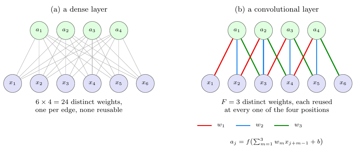
Figure 10.1: The two structural assumptions of Section Why not simply use a dense layer?, drawn on a one-dimensional input of six components. (a) A dense layer connects every input to every output and gives each edge its own weight. (b) A convolutional layer with \(F=3\) connects each output to a window of three neighbouring inputs – that is locality – and uses the same three weights \(w_1,w_2,w_3\) at every position, drawn here in the same three colours – that is parameter sharing. Twenty-four weights become three, and the three do not grow when the input is lengthened. Both pictures use the layer notation of Section Notation and the feed-forward pass: panel (a) is one layer of Figure 8.5.
10.2. Convolution#
For two functions on the real line the convolution is
where \(x\) is called the input and \(w\) the kernel, filter or weight function. The discrete version, which is what we shall use throughout, replaces the integral by a sum,
In practice \(w\) has only finitely many non-zero entries, say \(w(0),\dots,w(m-1)\), and the sum is finite.
Two elementary properties will be used repeatedly. Convolution is commutative, \(x*w=w*x\), which follows from the substitution \(k\to i-k\) in Eq. (10.4); and it is linear in each argument separately. Linearity is what allows a convolution to be written as a matrix, which we do next.
10.2.1. Convolution is polynomial multiplication#
The quickest route to intuition is an example that has nothing to do with images. Take two polynomials
whose product is a polynomial of degree five, \(z(t)=\sum_{l=0}^{5}\delta_l t^{l}\). Collecting terms,
Every line has the same shape: the indices of the two factors sum to the index of the result. That is precisely Eq. (10.4),
Polynomial multiplication is discrete convolution. This is not an analogy; the coefficient sequences convolve.
10.2.2. Toeplitz structure#
Since Eq. (10.7) is linear in \(\bm{\beta}\) we may write it as a matrix acting on \(\bm{\beta}\). Reading off the coefficients of Eq. (10.6),
Because convolution is commutative the same vector is obtained from \(\bm{T}_{\beta}\bm{\alpha}\) with a \(6\times3\) matrix built from \(\bm{\beta}\); which of the two sequences is called the filter is a matter of interpretation, not of mathematics.
The matrix in Eq. (10.8) has a name.
Definition 10.1 (Toeplitz matrix)
A matrix \(\bm{A}\in\mathbb{R}^{p\times q}\) is Toeplitz if its entries depend only on the difference of the indices,
equivalently if \(A_{i+1,j+1}=A_{ij}\) whenever both are defined. Each descending diagonal is constant. A Toeplitz matrix need not be square.
Theorem 10.2 (Convolution and Toeplitz matrices)
Let \(w\in\mathbb{R}^{m}\) and \(x\in\mathbb{R}^{n}\). The linear map \(x\mapsto w*x\) from \(\mathbb{R}^{n}\) to \(\mathbb{R}^{n+m-1}\) is represented by the Toeplitz matrix \(\bm{T}_w\in\mathbb{R}^{(n+m-1)\times n}\) with \((\bm{T}_w)_{ij}=w_{i-j}\), where \(w_k\equiv0\) outside \(0\le k\le m-1\). Conversely, every Toeplitz matrix arises this way. A matrix therefore represents a convolution if and only if it is Toeplitz.
Proof
The \(i\)th component of \(w*x\) is \(\sum_k w_k x_{i-k}\). Substituting \(j=i-k\) gives \(\sum_j w_{i-j}x_j\), which is the \(i\)th component of \(\bm{T}_w\bm{x}\) with \((\bm{T}_w)_{ij}=w_{i-j}\); this satisfies Definition 10.1 by construction. For the converse, given Toeplitz \(\bm{A}\) with \(A_{ij}=a_{i-j}\), set \(w_k=a_k\); then \((\bm{A}\bm{x})_i=\sum_j a_{i-j}x_j=(w*x)_i\).
Theorem 10.2 is worth pausing on, because it says the two structural assumptions of Section Why not simply use a dense layer? are not merely convenient but exhaustive. Locality makes the matrix banded; parameter sharing makes each diagonal constant; and a banded matrix with constant diagonals is a Toeplitz matrix, which is a convolution. There is no third option. Figure 10.3(a) shows such a matrix.
Do not build these matrices
The Toeplitz form is for reasoning, not for computing. Storing \(\bm{T}_w\) costs \(\bigO(n^{2})\) and multiplying by it costs \(\bigO(n^{2})\) operations, whereas evaluating Eq. (10.4) directly costs \(\bigO(nm)\) with \(m\ll n\), and \(\bigO(n\log n)\) by the fast Fourier transform, since convolution in the spatial domain is multiplication in the frequency domain. The code in Section Implementation from scratch never forms a Toeplitz matrix.
10.2.3. Diagonalisation: the convolution theorem#
The notebox above claimed that a convolution costs \(\bigO(n\log n)\) by the fast Fourier transform because convolution in one domain is multiplication in the other. That claim is a theorem about the eigenvectors of the Toeplitz structure, and it is worth proving, both because it is the reason the fast algorithms exist and because it is the cleanest illustration in this book of the principle of Chapter 1: a matrix is easy to work with in the basis of its own eigenvectors.
Take the periodic case, in which indices wrap modulo \(n\). The Toeplitz matrix of Definition 10.1 then becomes circulant: each row is the previous row shifted one place to the right, and \(C_{ij}=c_{(i-j)\bmod n}\).
Theorem 10.3 (Circular convolution is diagonalised by the DFT)
Let \(\bm{C}\) be the circulant matrix generated by \(\bm{c}\in\mathbb{C}^{n}\) and let \(\bm{F}\) be the discrete Fourier matrix, \(F_{kj}=n^{-1/2}\omega^{-kj}\) with \(\omega=e^{2\pi i/n}\). Then
so that every circulant matrix has the same eigenvectors – the Fourier modes – and eigenvalues given by the discrete Fourier transform of its generating vector. Consequently
the convolution theorem: convolution becomes elementwise multiplication.
Proof
Let \(\bm{v}_k\) have components \((\bm{v}_k)_j=\omega^{kj}\), the \(k\)th Fourier mode. Then
where the substitution \(m=(i-j)\bmod n\) is a bijection of \(\{0,\dots,n-1\}\) onto itself and the periodicity of \(\omega\) removes the modulus. So \(\bm{v}_k\) is an eigenvector with eigenvalue \(\hat{c}_k\), for every \(k\); the \(\bm{v}_k\) are orthogonal and \(n^{-1/2}\bm{v}_k\) are the columns of \(\bm{F}^{*}\), which is Eq. (10.10). Equation (10.11) follows by applying \(\bm{F}\) to \(\bm{C}\bm{x}\) and reading off the diagonal.
Three consequences follow immediately, and each is used somewhere later in this book. Computationally, Eq. (10.11) says a convolution costs two transforms and \(n\) multiplications, so \(\bigO(n\log n)\) rather than \(\bigO(n^{2})\); this is how large kernels are actually applied. Structurally, all circulant matrices commute, since they are simultaneously diagonalised – which is the algebraic content of the statement that convolutions compose into convolutions. And conceptually, Eq. (10.10) says a convolutional layer acts on each Fourier mode independently, multiplying it by a single learned number: a convolutional network is a learned filter bank, and what it learns is a frequency response.
Why the theorem does not simply end the chapter
If convolution is elementwise multiplication in Fourier space, why not build networks there and skip the spatial domain? Because the kernels used in practice are tiny. With \(F=3\) the direct cost is \(9n\) operations against \(\bigO(n\log n)\) for two transforms plus the product, and the crossover on typical image sizes is around \(F\approx11\). More fundamentally, the non-linearity between layers is elementwise in space, and an elementwise operation in one domain is a convolution in the other – so the network cannot stay in either domain. The architecture alternates between a map that is diagonal in frequency and a map that is diagonal in space, and that alternation is where its expressive power comes from.
10.2.4. Padding, and why indices go out of range#
Rename \(\bm{\alpha}\) as the filter \(\bm{w}\), of length \(m\), and \(\bm{\beta}\) as the input \(\bm{x}\), of length \(n\), with \(m\le n\). Then
For \(i=0\) this requires \(x(-1)\) and \(x(-2)\), which do not exist, and for \(i=n+m-2\) it requires indices past the end. The standard remedy is padding: extend \(\bm{x}\) with \(P\) zeros at each end, so that its length becomes \(n+2P\). With \(P=m-1\) every index in Eq. (10.12) is defined and the output has full length \(n+m-1\); this is called full padding. Two other choices are used constantly: \(P=0\), or valid padding, which evaluates the sum only where it is defined and shrinks the output to \(n-m+1\); and \(P=(m-1)/2\) for odd \(m\), or same padding, which returns an output of exactly length \(n\).
Padding with zeros is a choice, and it is visible in the result: outputs near the boundary are computed from fewer genuine inputs than outputs in the interior, so a padded convolution treats the border differently from the middle. Reflecting or wrapping the signal instead are common alternatives.
10.2.5. Cross-correlation, which is what libraries actually compute#
Equation (10.4) contains \(x(i-k)\): as \(k\) increases the input is read backwards. Implementing this means flipping the kernel before sliding it, which is a nuisance and, when the kernel is learned rather than prescribed, entirely pointless. Every deep learning library therefore computes
the cross-correlation, while calling it convolution. We follow the same convention from here on.
Why the distinction does not matter here, and when it does
Cross-correlation with \(w\) equals convolution with the reflected kernel \(\tilde{w}(k)=w(-k)\). Since \(w\) is learned, the network simply learns the reflected filter, and the set of functions the layer can represent is identical. The distinction matters only when the kernel is prescribed rather than learned – a Gaussian blur, a derivative filter, a matched filter from signal processing – or when comparing against a formula from a textbook that uses the true convolution. Note also that cross-correlation is not commutative, so the symmetry between filter and input in Eq. (10.8) is lost.
10.3. Two dimensions, channels and the convolutional layer#
For a two-dimensional input \(\bm{X}\) and kernel \(\bm{W}\) the definition extends in the obvious way,
and in the cross-correlation form actually used,
Real inputs have a channel axis, and a layer produces several outputs called feature maps. Let the input be \(\bm{X}\in\mathbb{R}^{C\times H\times W}\) with \(C\) channels, and let there be \(K\) filters, each of shape \(C\times F\times F\), collected in \(\bm{W}\in\mathbb{R}^{K\times C\times F\times F}\) with biases \(\bm{b}\in\mathbb{R}^{K}\). The layer computes, for \(k=0,\dots,K-1\),
followed by an elementwise activation, \(A=f(Z)\). Here \(S\) is the stride, the step by which the filter is moved, and \(P\) the padding.
Three points about Eq. (10.16) deserve emphasis. The sum over \(c\) runs over all input channels: a filter is not applied channel by channel but sees the full depth at each spatial location, which is why its shape is \(C\times F\times F\) and not \(F\times F\). The indices \(i,j\) range over output positions while \(m,n\) range over the filter, so the filter is small and the output is large. And \(W\) does not depend on \(i\) or \(j\) – that is parameter sharing, written out. Figure 10.2 shows the three statements as one picture: a filter drawn as a block spanning the full depth, one output value produced from it, and the \(K\) maps that \(K\) such filters make.
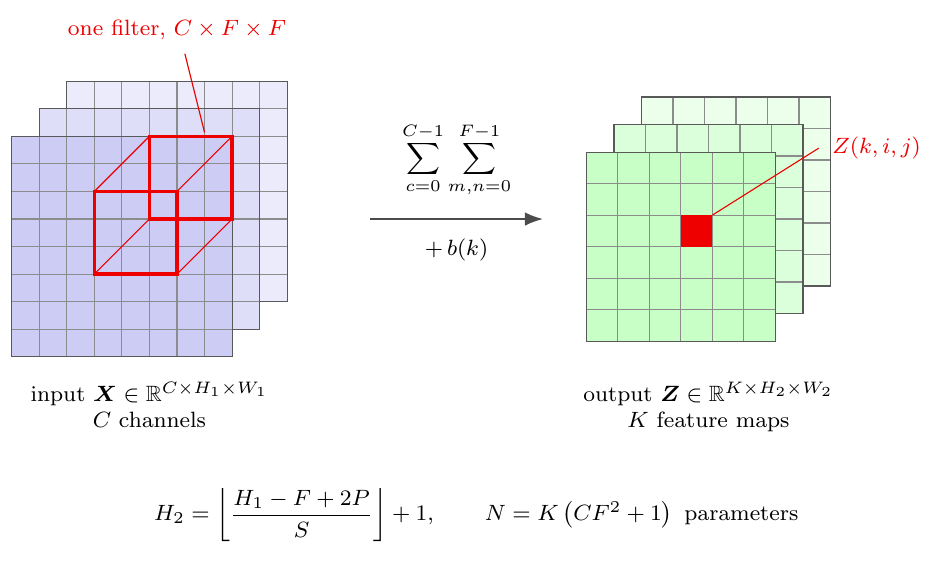
Figure 10.2: Equation (10.16) drawn. A filter is a \(C\times F\times F\) block, not an \(F\times F\) patch: it spans the whole depth of the input at each spatial location, which is why the sum over \(c\) in Eq. (10.16) has no counterpart among the output indices. The block shown produces the single value \(Z(k,i,j)\) marked in the output; sliding it over all positions \((i,j)\) with step \(S\) fills one feature map, and using \(K\) different filters produces the \(K\) maps stacked behind it. The spatial sizes follow Proposition 10.4 and the parameter count is independent of \(H_1\) and \(W_1\).
10.3.1. Output size and parameter count#
Proposition 10.4 (Convolution arithmetic)
Let the input have height \(H_1\), width \(W_1\) and depth \(C\), and apply \(K\) filters of spatial extent \(F\) with stride \(S\) and padding \(P\). Then the output volume has depth \(D_2=K\) and spatial dimensions
and the layer has
trainable parameters.
Proof
Along the height, the padded input has \(H_1+2P\) entries. The filter occupies positions \(0,S,2S,\dots\) and its last element must not run past the end, so the largest admissible starting index \(t\) satisfies \(t+F-1\le H_1+2P-1\), that is \(t\le H_1+2P-F\). The number of admissible multiples of \(S\) in \([0,H_1+2P-F]\) is \(\lfloor(H_1+2P-F)/S\rfloor+1\), which is Eq. (10.17); the width is identical. Each output channel is produced by one filter of \(CF^{2}\) weights plus one bias, and there are \(K\) of them, giving Eq. (10.18).
The floor in Eq. (10.17) is not decoration. When \(S\) does not divide \(H_1+2P-F\) the filter cannot reach the last few rows, and they are silently discarded. Choosing \(F\), \(S\) and \(P\) so that the division is exact is the reason for the familiar combinations \(F=3,S=1,P=1\) and \(F=5,S=1,P=2\), both of which give \(H_2=H_1\).
Example 10.5 (A concrete count)
An input volume of \(32\times32\times3\) with \(K=10\) filters of extent \(F=5\), stride \(S=1\) and padding \(P=0\) gives \(H_2=W_2=(32-5)/1+1=28\), so the output is \(28\times28\times10\). Each filter has \(5\times5\times3=75\) weights and one bias, so the layer has \(10\times76=760\) parameters. A dense layer with the same number of outputs would have \(3072\times7840\approx2.4\times10^{7}\).
10.3.2. The unrolled matrix#
Equation (10.16) is linear in \(\bm{X}\), so it must be a matrix. Take the small example of a \(3\times3\) input and a \(2\times2\) filter with \(S=1\), \(P=0\). Flattening the input row by row into \(\bm{X}'\in\mathbb{R}^{9}\) and the output into \(\bm{Y}'\in\mathbb{R}^{4}\), the convolution is \(\bm{Y}'=\bm{W}'\bm{X}'\) with
This matrix is doubly block Toeplitz: it is a Toeplitz matrix whose entries are themselves Toeplitz blocks, the outer structure coming from the row index and the inner from the column index. Four numbers appear in thirty-six positions. We verify this claim numerically in Section Implementation from scratch by reconstructing \(\bm{W}'\) column by column from the implementation and checking that it has exactly sixteen non-zero entries taking exactly four distinct values; Figure 10.3(b) shows the same pattern for a \(5\times5\) input and a \(3\times3\) kernel.
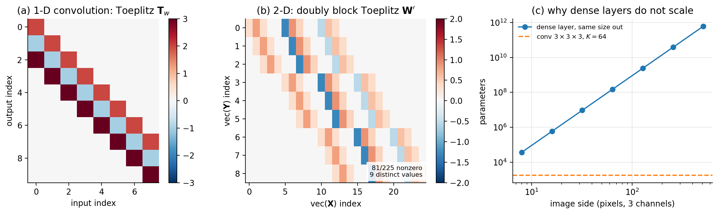
Figure 10.3: Convolution as a structured sparse matrix. (a) A one-dimensional convolution with a kernel of length three acting on an input of length eight, Eq. (10.8); each descending diagonal is constant, which is Definition 10.1. (b) The doubly block Toeplitz matrix \(\bm{W}'\) of Eq. (10.19) for a \(5\times5\) input and a \(3\times3\) kernel, reconstructed column by column from the code of Section Implementation from scratch: nine distinct numbers fill eighty-one of two hundred and twenty-five positions. (c) Parameters in a single layer as a function of image side, Eqs. (10.1) and (10.2); the dense layer grows as \(L^{4}\) while the convolutional layer does not grow at all.
10.4. Equivariance, and what it does and does not give#
Sparsity and parameter sharing explain the parameter count. The property that explains why convolution is the right restriction, rather than merely a cheap one, is equivariance.
Definition 10.6 (Equivariance and invariance)
Let \(T_s\) denote translation by \(s\), \((T_s x)(i)=x(i-s)\). A map \(\Phi\) is equivariant to translation if
and invariant if \(\Phi(T_s x)=\Phi(x)\) for all \(x,s\).
Equivariance says that translating the input translates the output by the same amount without otherwise changing it: if a filter responds to an edge, it responds to that edge wherever the edge moves. Invariance says the output does not move at all. Both are wanted, but at different places in the network: equivariance in the convolutional layers, where we want to know where features are, and invariance at the end, where we want to know only what the image contains.
Theorem 10.7 (Convolution is exactly the equivariant linear map)
Let \(\Phi:\mathbb{R}^{\mathbb{Z}}\to\mathbb{R}^{\mathbb{Z}}\) be linear. Then \(\Phi\) is equivariant to all translations if and only if \(\Phi\) is a convolution, that is, there is a \(w\) with \(\Phi(x)=w*x\).
Proof
(\(\Leftarrow\)) With \(\Phi(x)=w*x\),
(\(\Rightarrow\)) Let \(\delta\) be the sequence with \(\delta(0)=1\) and \(\delta(i)=0\) otherwise, and put \(w=\Phi(\delta)\), the impulse response. Any \(x\) may be written \(x=\sum_s x(s)\,T_s\delta\). By linearity and then equivariance,
whose \(i\)th component is \(\sum_s x(s)w(i-s)=(w*x)(i)\).
This is the theorem that justifies the architecture. We did not choose convolution from a menu of plausible local operations; once we demand a linear map that commutes with translation, convolution is the only thing left. The restriction from \(\bigO(L^{4})\) parameters to \(\bigO(F^{2})\) is the exact price of that symmetry.
Two qualifications matter in practice, and both are easy to state and easy to forget.
Proposition 10.8 (Stride breaks equivariance)
A convolution with stride \(S\) is equivariant to translations by multiples of \(S\) only. For \(s\) not divisible by \(S\), in general \(\Phi(T_sx)\neq T_{\lfloor s/S\rfloor}\Phi(x)\).
Proof
Striding retains outputs at positions \(Si\). Shifting the input by \(s\) shifts the underlying full-stride output by \(s\), and the retained subset \(\{Si\}\) maps to \(\{Si+s\}\), which coincides with \(\{Si\}\) as a set if and only if \(S\mid s\). Otherwise a different subsample of the same signal is retained and no translation of the output reproduces it.
We confirm this numerically in Section Implementation from scratch: for \(S=1\) the equivariance error is exactly zero, for \(S=2\) it is exactly zero for even shifts and \(\bigO(1)\) for odd ones. Padding is the second qualification. With zero padding the boundary rows are computed from invented zeros, so equivariance holds in the interior but fails within \(F/2\) of the edge – which is why the numerical check in Section Implementation from scratch is stated on the interior.
Figure 10.4 shows the property directly.
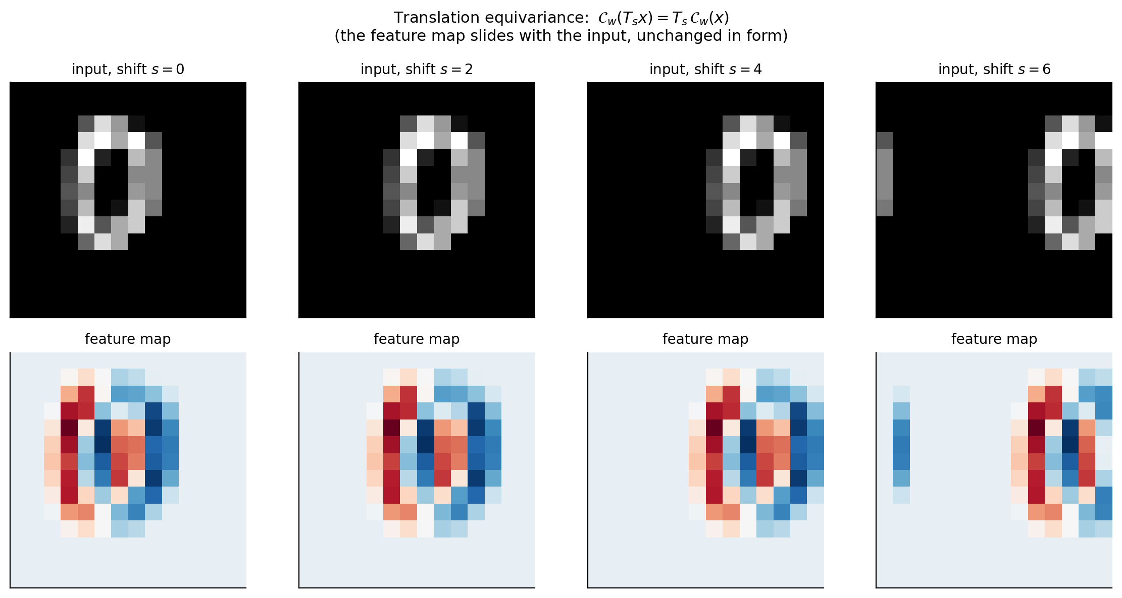
Figure 10.4: Translation equivariance, Eq. (10.20), for a fixed \(3\times3\) derivative filter applied to a digit placed at four positions on a \(14\times14\) canvas. The feature map in the lower row slides with the input in the upper row and is otherwise unchanged: measured on the interior, the discrepancy \(\max|\mathcal{C}_w(T_sx)-T_s\mathcal{C}_w(x)|\) is exactly zero. A dense layer has no such property, and must learn each position separately.
10.5. Pooling#
Equivariance propagates information about position through the network. At some point we want to discard it: a classifier should report “digit three” regardless of where the three sat. Pooling is the operation that trades position for robustness.
A pooling layer slides a window of size \(F\) with stride \(S\) over each channel independently and applies a fixed function to the contents. Max pooling,
is by far the most common; average pooling replaces the maximum by the mean. Pooling has no trainable parameters, and it does not mix channels, so the depth is unchanged and Eq. (10.17) governs the spatial sizes with \(P=0\).
The usual choice \(F=S=2\) discards three quarters of the activations in one step, as in Figure 10.5. The gain is a limited invariance: if the largest value in a window moves within that window, the output does not change at all. Pooling therefore converts equivariance at fine scale into invariance at fine scale, and stacking convolution and pooling alternately builds up invariance to progressively larger displacements while the receptive field grows.
Proposition 10.9 (Local invariance of max pooling)
Let \(\Pi\) be max pooling with window \(F\) and stride \(S=F\), so that the windows tile the input without overlap, and let \(x\) be supported in one window \(\mathcal{W}\). If \(T_s x\) is still supported in \(\mathcal{W}\), then \(\Pi(T_sx)=\Pi(x)\). If instead \(s\) moves the support into the neighbouring window, the output is unchanged in value but appears one position later.
Proof
The pooling output at window \(\mathcal{W}\) is \(\max_{p\in\mathcal{W}}x(p)\), which depends on the multiset of values in \(\mathcal{W}\) and not on their arrangement; a translation that permutes positions within \(\mathcal{W}\) therefore leaves it fixed. A translation carrying the support into the next window leaves the multiset intact but attaches it to the next output index.
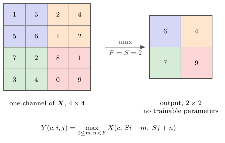
Figure 10.5: Max pooling with \(F=S=2\), Eq. (10.21). The four non-overlapping windows are shaded in four colours and each contributes one value, its maximum, to the correspondingly shaded output cell. Three quarters of the activations are discarded and nothing is learned: the operation has no parameters at all. Proposition 10.9 is visible here – move the \(9\) anywhere within its own window and the output is unchanged, move it into a neighbouring window and the output merely shifts.
Proposition 10.9 is the precise version of “a limited invariance”. Pooling is exactly invariant to displacements that stay inside a window and merely equivariant to larger ones – so a stack of pooling layers buys invariance to displacements up to the size of the last window measured in input pixels, and no more. That quantity is the receptive field, which we now compute.
Proposition 10.10 (Receptive field)
Consider \(L\) layers, layer \(\ell\) having filter size \(F_\ell\) and stride \(S_\ell\). The receptive field \(R_L\) of one output unit – the number of input pixels along one axis that can influence it – satisfies \(R_0=1\) and
Proof
A unit at layer \(\ell\) draws on \(F_\ell\) consecutive units of layer \(\ell-1\), whose receptive fields are each of size \(R_{\ell-1}\) and are offset from one another by the cumulative stride \(\prod_{j<\ell}S_j\) measured in input pixels. The union of \(F_\ell\) intervals of length \(R_{\ell-1}\) spaced by that offset has length \(R_{\ell-1}+(F_\ell-1)\prod_{j<\ell}S_j\).
Equation (10.22) explains a design rule. With \(3\times3\) filters and unit stride the receptive field grows only as \(2\ell+1\), painfully slowly; every pooling layer of stride two doubles the multiplier and the growth becomes geometric. Three blocks of two \(3\times3\) convolutions followed by a \(2\times2\) pool reach a receptive field of \(R=44\), enough to see most of a \(32\times32\) image. Stacking small filters rather than using one large one is also cheaper: two \(3\times3\) layers have receptive field \(5\) and \(2\times9C^2\) weights, against \(25C^2\) for a single \(5\times5\) layer, and they include an extra non-linearity.
10.5.1. Dilation: receptive field without cost#
Equation (10.22) shows two ways to enlarge the receptive field, and both are expensive: larger filters cost \(\bigO(F^{2})\) parameters, and stride or pooling costs resolution. A third way costs neither. A dilated or atrous convolution with rate \(D\) spreads the filter taps apart,
which for \(D=1\) is Eq. (10.15) and for \(D>1\) reads from a grid of the same \(F^{2}\) positions spaced \(D\) apart.
Proposition 10.11 (Effective filter size and dilated receptive field)
A dilated convolution with filter size \(F\) and rate \(D\) has the same \(K(CF^{2}+1)\) parameters as an undilated one and an effective filter size
Stacking \(L\) such layers with unit stride and rates \(D_\ell\) gives a receptive field
In particular, \(F=3\) with \(D_\ell=2^{\ell-1}\) gives \(R_L=2^{L+1}-1\): the receptive field grows exponentially in depth while the parameter count grows linearly and the resolution is never reduced.
Proof
The taps occupy positions \(0,D,2D,\dots,D(F-1)\), spanning \(D(F-1)+1\) pixels, which is Eq. (10.24); the number of taps, and hence of weights, is unchanged. Substituting \(F_\ell\to D_\ell(F_\ell-1)+1\) into Eq. (10.22) with all \(S_j=1\) gives \(R_\ell = R_{\ell-1}+D_\ell(F_\ell-1)\), and summing from \(R_0=1\) gives Eq. (10.25). With \(F_\ell=3\) and \(D_\ell=2^{\ell-1}\) the sum is \(1+2\sum_{\ell=1}^{L}2^{\ell-1}=2^{L+1}-1\).
Compare the three routes to a receptive field of \(R=63\) with \(3\times3\) filters. Unit stride and no dilation needs \(31\) layers, by \(R=2L+1\). Pooling of stride two every second layer needs about \(10\) and throws away a factor of \(32\) in resolution. Exponential dilation needs \(5\), by Proposition 10.11, at full resolution throughout. This is why dilation is standard in segmentation, where the output must have the same size as the input, and in the audio models where the receptive field must span thousands of samples. Figure 10.6 shows both cases for two layers, with the reach of a single output unit shaded on the input row.
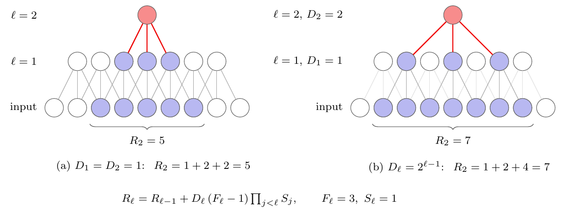
Figure 10.6: The receptive field of Proposition 10.10 and what dilation does to it, for two layers of \(F=3\) with unit stride. The shaded input units are those the single top unit can see. (a) Without dilation the two layers reach five inputs, and Eq. (10.22) gives the familiar \(R_\ell=2\ell+1\). (b) With \(D_2=2\) the second layer reads every other unit of the first – the pale edges are first-layer units that are computed but not read by this particular output – and the reach becomes seven. The filter has the same three taps in both panels and the resolution is reduced in neither; Proposition 10.11 continues the pattern to \(R_L=2^{L+1}-1\).
10.6. Backpropagation through a convolutional layer#
Chapter 8 derived the four equations of backpropagation for dense layers. Nothing about them changes here – the network is still a composition of differentiable maps and the chain rule is still the chain rule – but the gradients of Eq. (10.16) are worth deriving explicitly, because the result is elegant and because the derivation is where errors hide.
Write \(\delta(k,i,j)=\partial\mathcal{C}/\partial Z(k,i,j)\) for the error propagated back to the output of the convolution, as in Chapter 8. We want \(\partial\mathcal{C}/\partial W\), \(\partial\mathcal{C}/\partial b\) and \(\partial\mathcal{C}/\partial X\).
The filter gradient. By the chain rule, summing over every output position that \(W(k,c,m,n)\) touched,
using Eq. (10.16) for the inner derivative. The right-hand side is itself a cross-correlation, of the input with the error. Every output position contributes to every filter weight: this is the price and the point of parameter sharing, and it is why a convolutional layer with few parameters can still receive a large, well-averaged gradient.
The bias gradient. Since \(b(k)\) is added at every spatial position of feature map \(k\),
The input gradient. Here we must collect every output that a given input pixel influenced,
where terms with filter indices outside \([0,F-1]\) are omitted. For \(S=1\) this is a convolution of \(\delta\) with the spatially flipped kernel – the transposed convolution – which is the cleanest way to remember it: the forward pass correlates, the backward pass convolves.
The backward pass is the adjoint
All three results are instances of one fact. The forward map \(\bm{X}\mapsto\bm{Z}\) is linear, represented by the matrix \(\bm{W}'\) of Eq. (10.19), so the gradient with respect to the input is \(\bm{W}'^{\top}\bm{\delta}\). Backpropagation through any linear layer is multiplication by its adjoint, and Eq. (10.28) is simply \(\bm{W}'^{\top}\) written out in index form. The code of Section Implementation from scratch exploits this directly, and we test it by checking the adjoint identity \(\langle\mathcal{A}\bm{x},\bm{y}\rangle =\langle\bm{x},\mathcal{A}^{*}\bm{y}\rangle\) numerically.
The transposed convolution. The remark that the backward pass is a convolution with the flipped kernel is worth promoting to a definition, because the same operation appears in the forward direction in every generative architecture of Part IV: the decoder of Chapter 15, the denoiser of Chapter 16 and the generator of Chapter 17 all have to enlarge a small array into a large one.
Proposition 10.12 (Transposed convolution)
Let \(\mathcal{A}\) be the convolution of Eq. (10.16) with filter size \(F\), stride \(S\) and padding \(P\), mapping an input of side \(H_1\) to an output of side \(H_2\) given by Eq. (10.17). Its adjoint \(\mathcal{A}^{*}\) – the map applied in the backward pass, and the layer called \verb!ConvTranspose2d! or \verb!Conv2DTranspose! – maps an array of side \(H_2\) to one of side
and is itself a convolution: for \(S=1\) it is the correlation with the spatially flipped kernel and padding \(F-1-P\), and for \(S>1\) it is the same after inserting \(S-1\) zeros between adjacent input elements.
Proof
Since \(\mathcal{A}\) is linear with matrix \(\bm{W}'\) as in Eq. (10.19), its adjoint has matrix \(\bm{W}'^{\top}\) and therefore maps \(\mathbb{R}^{H_2\times H_2}\to\mathbb{R}^{H_1\times H_1}\); solving Eq. (10.17) for \(H_1\) in the case where \(S\) divides \(H_1+2P-F\) gives Eq. (10.29). For the second statement, Eq. (10.28) with \(S=1\) reads \(\partial\mathcal{C}/\partial X(c,p,q)=\sum_k\sum_{i,j}\delta(k,i,j) W(k,c,p-i+P,q-j+P)\), which is the correlation of \(\delta\) with \(W\) read in reverse index order, that is with the flipped kernel, and the index range requires \(F-1-P\) zeros of padding on \(\delta\). For \(S>1\), Eq. (10.28) has \(\delta\) evaluated only at positions \(Si\), which is \(\delta\) upsampled by inserting \(S-1\) zeros.
Equation (10.29) is the formula to reach for when a generator has to be designed backwards from its output size, and the zero insertion is the reason transposed convolutions produce the checkerboard artefacts that are visible in early GAN samples: neighbouring output pixels are computed from different numbers of genuine inputs when \(S\) does not divide \(F\). Choosing \(F\) a multiple of \(S\) – \(F=4\), \(S=2\) is the usual pair, and is what Chapter 17 uses – removes them.
Through a pooling layer. Max pooling is not differentiable everywhere, but it is differentiable almost everywhere, and where it is the derivative is a routing:
The gradient flows only to the element that won the maximum, and the argmax must be recorded during the forward pass. Ties have measure zero and are broken arbitrarily. For average pooling the gradient is instead spread equally, each of the \(F^{2}\) inputs receiving \(\delta/F^{2}\).
10.7. Implementation from scratch#
We now write the whole thing in NumPy, in the same style as Chapter 8: parameters are plain arrays, the forward pass is a function, and every gradient is checked against finite differences before anything is trained.
10.7.1. The im2col transformation#
The six nested loops implied by Eq. (10.16) are correct and unusably slow in Python. The standard remedy is im2col: rearrange every \(F\times F\) patch of the input into a column, so that the convolution becomes a single matrix product. If \(\bm{X}\) has shape \((N,C,H,W)\), the result has shape \((N,\,CF^{2},\,H_2W_2)\) and
which BLAS executes at full speed. The cost is memory: each input element is replicated up to \(F^{2}\) times.
def im2col(X, F, S, P):
    """Rearrange every F x F patch of X into a column, Eq. (10.im2col).

    X has shape (N, C, H, W); the result has shape (N, C*F*F, H2*W2) with
    H2 = (H - F + 2P)/S + 1, so that a convolution becomes one matrix product.
    """
    N, C, H, W = X.shape
    H2 = (H - F + 2 * P) // S + 1
    W2 = (W - F + 2 * P) // S + 1
    Xp = pad2d(X, P)
    cols = np.empty((N, C * F * F, H2 * W2))
    for i in range(F):
        for j in range(F):
            patch = Xp[:, :, i:i + S * H2:S, j:j + S * W2:S]      # (N,C,H2,W2)
            cols[:, (i * F + j)::F * F, :] = patch.reshape(N, C, -1)
    return cols


def col2im(cols, X_shape, F, S, P):
    """Adjoint of im2col: scatter columns back, accumulating overlaps."""
    N, C, H, W = X_shape
    H2 = (H - F + 2 * P) // S + 1
    W2 = (W - F + 2 * P) // S + 1
    Xp = np.zeros((N, C, H + 2 * P, W + 2 * P))
    for i in range(F):
        for j in range(F):
            patch = cols[:, (i * F + j)::F * F, :].reshape(N, C, H2, W2)
            np.add.at(Xp, (slice(None), slice(None),
                           slice(i, i + S * H2, S), slice(j, j + S * W2, S)), patch)
    return Xp if P == 0 else Xp[:, :, P:-P, P:-P]
The loops run over the filter, which is small, not over the image. The forward and backward passes follow directly from Eqs. (10.26)–(10.28).
def conv_forward(X, W, b, S=1, P=0):
    """Cross-correlation, Eq. (10.crosscorr2d).  W has shape (K, C, F, F)."""
    N, C, H, Wd = X.shape
    K, _, F, _ = W.shape
    H2 = (H - F + 2 * P) // S + 1
    W2 = (Wd - F + 2 * P) // S + 1
    cols = im2col(X, F, S, P)                       # (N, C*F*F, H2*W2)
    out = np.einsum("kd,ndp->nkp", W.reshape(K, -1), cols) + b[None, :, None]
    return out.reshape(N, K, H2, W2), cols


def conv_backward(dY, X, W, cols, S=1, P=0):
    """Gradients of the convolution, Eqs. (10.dconvW), (10.dconvb), (10.dconvX)."""
    N, K, H2, W2 = dY.shape
    _, C, F, _ = W.shape
    dYf = dY.reshape(N, K, -1)                                   # (N,K,H2W2)
    dW = np.einsum("nkp,ndp->kd", dYf, cols).reshape(W.shape)
    db = dYf.sum(axis=(0, 2))
    dcols = np.einsum("kd,nkp->ndp", W.reshape(K, -1), dYf)
    dX = col2im(dcols, X.shape, F, S, P)
    return dX, dW, db
Max pooling stores the argmax so that Eq. (10.30) can route the gradient:
def maxpool_forward(X, F=2, S=2):
    """Max pooling, Eq. (10.maxpool).  Returns the output and an argmax mask."""
    N, C, H, W = X.shape
    H2, W2 = (H - F) // S + 1, (W - F) // S + 1
    patches = np.empty((N, C, H2, W2, F * F))
    for i in range(F):
        for j in range(F):
            patches[..., i * F + j] = X[:, :, i:i + S * H2:S, j:j + S * W2:S]
    idx = patches.argmax(axis=-1)
    out = np.take_along_axis(patches, idx[..., None], axis=-1)[..., 0]
    return out, idx


def maxpool_backward(dY, X, idx, F=2, S=2):
    """Route each gradient to the argmax that produced it, Eq. (10.dmaxpool)."""
    N, C, H, W = X.shape
    H2, W2 = dY.shape[2], dY.shape[3]
    dX = np.zeros_like(X)
    for i in range(F):
        for j in range(F):
            mask = (idx == i * F + j)
            np.add.at(dX, (slice(None), slice(None),
                           slice(i, i + S * H2, S), slice(j, j + S * W2, S)),
                      dY * mask)
    return dX
10.7.2. Verifying the implementation#
Four checks, in increasing order of strength. First, that \verb!conv_forward! agrees with the definition (10.16) coded as an explicit quadruple loop, for several strides and paddings:
S=1 P=0  shape (2, 4, 5, 5)  max|conv-naive| = 3.553e-15
S=1 P=1  shape (2, 4, 7, 7)  max|conv-naive| = 3.553e-15
S=2 P=1  shape (2, 4, 4, 4)  max|conv-naive| = 3.553e-15
S=2 P=0  shape (2, 4, 3, 3)  max|conv-naive| = 1.776e-15
S=3 P=2  shape (2, 4, 3, 3)  max|conv-naive| = 2.220e-15
Second, the adjoint identity of the notebox in Section Backpropagation through a convolutional layer, \(\langle\mathrm{im2col}(\bm{x}),\bm{y}\rangle =\langle\bm{x},\mathrm{col2im}(\bm{y})\rangle\), which must hold to rounding:
F=3 S=1 P=0:  |<Ax,y>-<x,A*y>| = 7.11e-15
F=3 S=2 P=1:  |<Ax,y>-<x,A*y>| = 4.44e-15
F=5 S=1 P=2:  |<Ax,y>-<x,A*y>| = 4.44e-15
Third, that the analytic gradients match central differences:
  S=1 P=0:  dX 9.73e-09   dW 7.76e-09   db 1.53e-09
  S=1 P=1:  dX 8.52e-09   dW 8.45e-09   db 5.43e-09
  S=2 P=1:  dX 4.94e-09   dW 5.36e-09   db 1.78e-09
  max-pool  dX 1.19e-09
Fourth, the structural claims of Sections Toeplitz structure and The unrolled matrix. Reconstructing \(\bm{W}'\) column by column from \verb!conv_forward! for the \(3\times3\) input and \(2\times2\) kernel reproduces Eq. (10.19) exactly: sixteen non-zero entries out of thirty-six, taking four distinct values, and \(\bm{W}'\bm{X}'=\mathrm{vec}(\bm{Y})\) to \(0.0\). The polynomial identity of Section Convolution is polynomial multiplication is confirmed by comparing the coefficients from \verb!polymul!, from \verb!np.convolve! and from \(\bm{T}_\alpha\bm{\beta}\), which agree exactly.
Equivariance, Theorem 10.7, and its failure under stride, Proposition 10.8, are equally sharp:
S=1 shift 1: max|conv(T_s x)-T_s conv(x)| = 0.00e+00
S=1 shift 2: max|conv(T_s x)-T_s conv(x)| = 0.00e+00
S=1 shift 3: max|conv(T_s x)-T_s conv(x)| = 0.00e+00
S=2 shift 1: max|.| = 7.119e+00   <- NOT equivariant
S=2 shift 2: max|.| = 0.000e+00   <- equivariant
You cannot naively gradient-check a ReLU and max-pool network
Running the finite-difference test on the full network of Section A complete network gives relative errors of \(10^{-8}\) for five of the six parameter arrays and a relative error of \(1.0\) – complete disagreement – for the first-layer bias \(\bm{b}_1\). This is not a bug. A bias shifts an entire feature map, so a perturbation of \(h=10^{-6}\) pushes some pre-activation across zero or changes which element wins a max-pool window. The network is piecewise linear, the central difference straddles a kink, and the two-sided quotient converges to nothing in particular. Repeating the same check with \(\tanh\) in place of ReLU and average in place of max pooling – smooth everywhere, same backward-pass code paths – gives
which is the finite-difference floor. The lesson is general: verify gradients on a smooth surrogate, then switch the activations back.
10.7.3. A complete network#
The layers assemble into the standard pattern, convolution and pooling alternating and a dense layer at the end:
The softmax and cross-entropy of Chapter 5 are unchanged, and so is the convenient identity \(\delta^{L}=(\bm{a}^{L}-\bm{y})/n\). Figure 10.7 draws the whole chain with the tensor shapes and parameter counts of the network we hand to PyTorch and Keras in Section The same network in PyTorch and TensorFlow, and it is worth looking at before reading the code: the shapes are the only thing that has to be got right, and every one of them follows from Proposition 10.4.
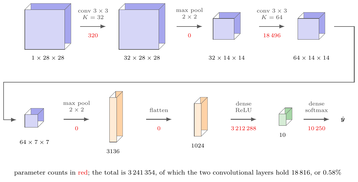
Figure 10.7: The pattern of Eq. (10.32), instantiated with the widths of the PyTorch and Keras listings of Section The same network in PyTorch and TensorFlow on MNIST, with \(F=3\), \(S=1\), \(P=1\) and \(2\times2\) pooling throughout; the dropout layer of Section Dropout, which has no parameters, is not drawn. Each slab is one tensor and is labelled with its shape; every spatial size follows Proposition 10.4 and every parameter count is the one checked against Keras in Section Parameter counts, checked. The shape of the picture is the argument of this chapter and its own refutation at once. The two convolutional layers, which carry all the locality, sharing and equivariance, hold \(18\,816\) of the \(3\,241\,354\) parameters; the single dense layer that follows the flattening, which has none of those properties, holds \(3\,212\,288\).
def forward(p, X):
    """Returns the class probabilities and everything the backward pass needs."""
    Z1, c1 = conv_forward(X, p["W1"], p["b1"], S=1, P=1)
    A1 = relu(Z1)
    P1, i1 = maxpool_forward(A1, 2, 2)
    Z2, c2 = conv_forward(P1, p["W2"], p["b2"], S=1, P=1)
    A2 = relu(Z2)
    P2, i2 = maxpool_forward(A2, 2, 2)
    flat = P2.reshape(P2.shape[0], -1)
    Z3 = flat @ p["W3"] + p["b3"]
    return softmax(Z3), (X, Z1, A1, i1, P1, c1, Z2, A2, i2, P2, flat, c2)


def backward(p, cache, probs, Y):
    """Backpropagation, Eqs. (10.dconvW)-(10.dmaxpool); delta^L = (a-y)/n."""
    X, Z1, A1, i1, P1, c1, Z2, A2, i2, P2, flat, c2 = cache
    n = X.shape[0]
    d3 = (probs - Y) / n                                    # softmax + CE
    g = {"W3": flat.T @ d3, "b3": d3.sum(axis=0)}
    dflat = d3 @ p["W3"].T
    dP2 = dflat.reshape(P2.shape)
    dA2 = maxpool_backward(dP2, A2, i2, 2, 2)
    dZ2 = dA2 * relu_prime(Z2)
    dP1, g["W2"], g["b2"] = conv_backward(dZ2, P1, p["W2"], c2, S=1, P=1)
    dA1 = maxpool_backward(dP1, A1, i1, 2, 2)
    dZ1 = dA1 * relu_prime(Z1)
    _, g["W1"], g["b1"] = conv_backward(dZ1, X, p["W1"], c1, S=1, P=1)
    return g
The initialisation is that of Chapter 8, with the observation that the fan-in of a convolutional filter is \(CF^{2}\) rather than the number of units in the previous layer:
def init_cnn(C_in=1, K1=8, K2=16, F=3, n_out=10, flat=None, rng=None):
    """He initialisation, Eq. (8.he), with fan-in C*F*F for a conv kernel."""
    rng = np.random.default_rng(0) if rng is None else rng
    def he(shape, fan_in):
        return rng.normal(0.0, np.sqrt(2.0 / fan_in), shape)
    return {
        "W1": he((K1, C_in, F, F), C_in * F * F), "b1": np.zeros(K1),
        "W2": he((K2, K1, F, F), K1 * F * F),     "b2": np.zeros(K2),
        "W3": he((flat, n_out), flat),            "b3": np.zeros(n_out),
    }
10.8. Does it actually help? An experiment#
The arguments of Sections Why not simply use a dense layer? and Equivariance, and what it does and does not give are arguments; this section measures. We use the \(8\times8\) handwritten digits shipped with scikit-learn, \(1797\) images, split \(70/30\), and compare the network of Eq. (10.32) against a dense network of the same size. Both are trained by Adam with \(\gamma=3\times10^{-3}\) for twenty epochs with batches of thirty-two, and every figure below is the mean over five random seeds.
\noalign{} Data |
Model |
Parameters |
Test accuracy |
|---|---|---|---|
\noalign{}\noalign{} centred \(8\times8\) |
CNN |
\(1898\) |
\(0.9656\) (\(0.9574\)–\(0.9704\)) |
centred \(8\times8\) |
dense |
\(1885\) |
\(0.9670\) (\(0.9593\)–\(0.9704\)) |
\noalign{}\noalign{} random offset \(12\times12\) |
CNN |
\(2698\) |
\(\mathbf{0.8774}\) (\(0.8574\)–\(0.9185\)) |
random offset \(12\times12\) |
dense |
\(6830\) |
\(0.7070\) (\(0.6815\)–\(0.7315\)) |
\noalign{} |
Table 10.1: Convolutional and dense networks compared on the scikit-learn digits. The upper block uses the images as supplied, centred in an \(8\times8\) frame; the lower block places the same digits at a uniformly random offset in a \(12\times12\) frame. Ranges are minimum and maximum over five seeds.
The first block is a negative result and we report it as such. On centred \(8\times8\) digits the convolutional network is not better: \(0.9656\) against \(0.9670\), a difference far smaller than the seed-to-seed spread of both. With matched parameter counts the two architectures are indistinguishable. This is not a failure of the implementation but a statement about the data. The digits are \(64\) pixels, pre-centred and pre-scaled; there is almost no translation for equivariance to exploit, and a dense layer can afford one weight per pixel per hidden unit. A reader who met CNNs only through MNIST-style demonstrations might reasonably conclude they are always better, and on this problem they are not.
The second block is where the argument lands. Placing the same digits at a random offset in a slightly larger frame – a change that a human classifier would not notice – costs the dense network twenty-six points of accuracy, from \(0.9670\) to \(0.7070\), while the convolutional network gives up nine, from \(0.9656\) to \(0.8774\). The CNN wins by seventeen points using \(2.5\) times fewer parameters, \(2698\) against \(6830\). The dense network must learn each digit separately at each of the twenty-five possible positions from a training set that contains only \(1257\) images; the convolutional network learns each feature once, by Theorem 10.7, and pooling supplies the tolerance to where it landed.
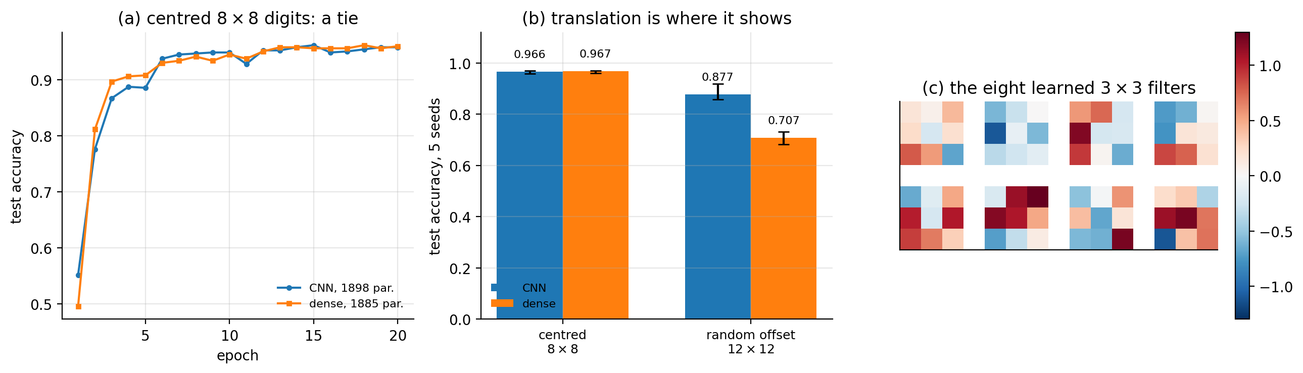
Figure 10.8: (a) Test accuracy against epoch on the centred digits for the two architectures of Table 10.1 at matched parameter count; the curves are on top of one another. (b) The same comparison on centred and randomly translated digits, bars showing the mean and whiskers the range over five seeds. Translation is what separates the two. (c) The eight \(3\times3\) first-layer filters after training: oriented opposed-sign pairs, which is to say edge detectors, learned rather than prescribed.
Panel (c) of Figure 10.8 is worth a glance. The first-layer filters, initialised at random and trained only against a classification loss, converge to small oriented patterns with a positive lobe beside a negative one. These are edge detectors of the kind that signal processing prescribes by hand, and nobody asked for them; they are what minimising cross-entropy on images produces.
10.9. Dropout#
The network we are about to hand to the libraries uses one ingredient we have not yet met. During training each unit is set to zero independently with probability \(p\),
where the factor \(1/(1-p)\) keeps \(\mathbb{E}[\tilde{a}_j]=a_j\) so that no rescaling is needed at test time, when dropout is switched off entirely. The effect is to prevent any unit from relying on the presence of any other, forcing the representation to be distributed rather than concentrated; it can also be read as training an ensemble of exponentially many subnetworks with shared weights, in the spirit of the bagging of Chapter 7.
Dropout is applied mainly after dense layers, where the parameters are and hence where overfitting is. Convolutional layers are already regularised by parameter sharing – a filter that overfits at one location would have to overfit identically everywhere – so dropout after a convolution is less common and often unhelpful.
10.10. The same network in PyTorch and TensorFlow#
Nothing above is a substitute for a library, and no serious work uses a NumPy convolution. The point of writing one was to know what the library is doing – and that is a claim we are now in a position to test rather than assert. This section gives the same architecture in both major frameworks, then loads one set of weights into all three implementations and compares them gradient by gradient, and finally trains the network on the sixty thousand MNIST images that the arithmetic of Section Output size and parameter count was always about.
10.10.1. PyTorch#
PyTorch expects tensors of shape \((N,C,H,W)\), the same layout as our NumPy code, and the layer
\verb!nn.Conv2d(C_in, K, F, padding=P)!
implements exactly Eq. (10.16). The example below is the MNIST network of the lecture notes, with two convolutional blocks, dropout and two dense layers.
import torch
import torch.nn as nn
import torch.nn.functional as F
import torch.optim as optim
from torchvision import datasets, transforms

device = torch.device("cuda" if torch.cuda.is_available() else "cpu")

transform = transforms.Compose([
    transforms.ToTensor(),
    transforms.Normalize((0.1307,), (0.3081,)),      # MNIST mean and std
])
train_set = datasets.MNIST(root="./data", train=True,  download=True,
                           transform=transform)
test_set  = datasets.MNIST(root="./data", train=False, download=True,
                           transform=transform)
train_loader = torch.utils.data.DataLoader(train_set, batch_size=64, shuffle=True)
test_loader  = torch.utils.data.DataLoader(test_set,  batch_size=64)


class CNN(nn.Module):
    """Eq. (10.arch) with two conv blocks; 28 -> 14 -> 7 by Eq. (10.outsize)."""
    def __init__(self):
        super().__init__()
        self.conv1 = nn.Conv2d(1, 32, 3, padding=1)   # 'same': 28 x 28
        self.conv2 = nn.Conv2d(32, 64, 3, padding=1)  # 'same': 14 x 14
        self.pool = nn.MaxPool2d(2, 2)                # halves each time
        self.fc1 = nn.Linear(64 * 7 * 7, 1024)
        self.fc2 = nn.Linear(1024, 10)
        self.dropout = nn.Dropout(0.5)

    def forward(self, x):
        x = self.pool(F.relu(self.conv1(x)))          # (N, 32, 14, 14)
        x = self.pool(F.relu(self.conv2(x)))          # (N, 64,  7,  7)
        x = x.view(-1, 64 * 7 * 7)
        x = self.dropout(F.relu(self.fc1(x)))
        return self.fc2(x)                            # logits, not probabilities


model = CNN().to(device)
criterion = nn.CrossEntropyLoss()      # applies softmax internally
optimizer = optim.Adam(model.parameters(), lr=1e-3)

for epoch in range(10):
    model.train()
    running = 0.0
    for data, target in train_loader:
        data, target = data.to(device), target.to(device)
        optimizer.zero_grad()
        loss = criterion(model(data), target)
        loss.backward()                # Eqs. (10.dconvW)-(10.dmaxpool), by autograd
        optimizer.step()
        running += loss.item()
    print(f"epoch {epoch+1}: loss {running/len(train_loader):.4f}")

model.eval()
correct = total = 0
with torch.no_grad():
    for data, target in test_loader:
        pred = model(data.to(device)).argmax(dim=1)
        correct += (pred == target.to(device)).sum().item()
        total += target.size(0)
print(f"test accuracy {100*correct/total:.2f}%")
Two details are easy to get wrong. \verb!nn.CrossEntropyLoss! expects logits and applies the softmax itself, so the network must not end with a softmax; applying one twice is a common and quiet bug. And \verb!model.train()! versus \verb!model.eval()! matters because of dropout, which is active only during training – at test time all units are used and the activations are rescaled to compensate.
10.10.2. TensorFlow and Keras#
Keras uses the opposite channel convention, \((N,H,W,C)\), and infers input shapes after the first layer.
import tensorflow as tf
from tensorflow.keras import datasets, layers, models

(train_images, train_labels), (test_images, test_labels) = datasets.mnist.load_data()
train_images = train_images.reshape((-1, 28, 28, 1)).astype("float32") / 255.0
test_images  = test_images.reshape((-1, 28, 28, 1)).astype("float32") / 255.0

model = models.Sequential([
    layers.Conv2D(32, (3, 3), padding="same", activation="relu",
                  input_shape=(28, 28, 1)),          # note channels LAST
    layers.MaxPooling2D((2, 2)),
    layers.Conv2D(64, (3, 3), padding="same", activation="relu"),
    layers.MaxPooling2D((2, 2)),
    layers.Flatten(),
    layers.Dense(1024, activation="relu"),
    layers.Dropout(0.5),
    layers.Dense(10),                                # logits
])

model.compile(optimizer=tf.keras.optimizers.Adam(1e-3),
              loss=tf.keras.losses.SparseCategoricalCrossentropy(from_logits=True),
              metrics=["accuracy"])
model.summary()          # prints Eq. (10.paramcount) layer by layer

model.fit(train_images, train_labels, epochs=10, batch_size=64,
          validation_data=(test_images, test_labels))
The flag \verb!from_logits=True! plays the role that \verb!nn.CrossEntropyLoss! plays in PyTorch. It is worth calling \verb!model.summary()! and checking the parameter counts against Eq. (10.18) by hand: the first layer should report \(32\times(1\times9+1)=320\) and the second \(64\times(32\times9+1)=18496\), while the dense layer that follows carries \(64\cdot7\cdot7\cdot1024+1024=3212288\). That last number is instructive. The two convolutional layers together hold \(18816\) parameters, less than one per cent of the network, and the dense layer holds almost all of it – which is why modern architectures replace the large dense layer with global average pooling.
10.10.3. Do the three implementations agree?#
The listings above and the NumPy code of Section Implementation from scratch are supposed to be the same function. Nothing so far has checked it, and there is more room for error than one might think: the three carry their arrays in different layouts, and a transposition that happens to be self-consistent will train perfectly well while computing something other than what is on the page. The conventions are
\noalign{} |
input |
kernel |
|---|---|---|
\noalign{}\noalign{} ours |
\((N,C,H,W)\) |
\((K,C,F,F)\) |
PyTorch |
\((N,C,H,W)\) |
\((K,C,F,F)\) |
Keras |
\((N,H,W,C)\) |
\((F,F,C,K)\) |
\noalign{} |
so ours and PyTorch agree and Keras differs in both. There is a third trap: our \verb!flatten! runs over \((K,H,W)\) in C order while Keras flattens \((H,W,K)\), so the rows of the dense weight matrix have to be permuted before they can be compared.
With all of that reconciled, we generate one set of weights, push it into all three, and evaluate the same eight real MNIST images. In double precision:
=== 1. one convolutional layer, identical weights ===
  output shape (N,K,H,W)      : (8, 4, 28, 28)
  max |ours  - torch|         : 1.332e-15
  max |ours  - keras|         : 1.776e-15
  max |torch - keras|         : 1.776e-15
  scale of the outputs        : 7.980

=== 3. the whole network of Eq. (10.arch), forward ===
  max |p_ours - p_torch|      : 3.053e-16
  max |p_ours - p_keras|      : 4.441e-16
  cross-entropy, ours         : 3.130017831683
  cross-entropy, torch        : 3.130017831724
  cross-entropy, keras        : 3.130017831724
The forward pass is settled. The interesting comparison is the backward one, because Eqs. (10.26)–(10.28) were derived by hand and the libraries obtain the same quantities by automatic differentiation, which shares no code and no reasoning with our derivation:
=== 4. the gradients of Section 10.convbackprop ===
   array      shape           |ours-torch|   |ours-keras|   scale
   W1     (4, 1, 3, 3)         2.082e-16     2.220e-16  4.05e-01
   b1     (4,)                 8.327e-17     2.776e-16  1.98e-01
   W2     (6, 4, 3, 3)         4.441e-16     4.441e-16  1.20e+00
   b2     (6,)                 8.327e-17     1.110e-16  2.69e-01
   W3     (294, 10)            3.331e-16     2.776e-16  6.38e-01
   b3     (10,)                5.551e-17     2.776e-17  2.46e-01
  worst disagreement anywhere : 4.441e-16
Every entry is at the double-precision rounding level, \(\epsilon\approx 2.2\times10^{-16}\), and the gradients themselves are of order one. Figure 10.9(b) plots the whole comparison against \(\epsilon\). The filter gradient (10.26), the bias gradient (10.27) and the input gradient (10.28) are what the frameworks compute; the derivation in Section Backpropagation through a convolutional layer is not a simplified account of it.
This is a stronger statement than the finite-difference check of Section Verifying the implementation. That check compared our gradient against our own forward pass, and would have passed even if both had implemented the wrong convolution. This one compares against two independent implementations written by other people.
10.10.4. Parameter counts, checked#
Running the arithmetic of Proposition 10.4 against what Keras reports for the network of the listings:
=== 5. parameter counts against Eq. (10.paramcount) ===
   layer                keras   K(C F^2 + 1) or n_in n_out + n_out
   conv2d(1->32)            320   32*(1*9+1) = 320
   conv2d(32->64)         18496   64*(32*9+1) = 18496
   dense(3136->1024)    3212288   3136*1024+1024 = 3212288
   dense(1024->10)        10250   1024*10+10 = 10250
   total                3241354
  the two convolutional layers hold 18816 parameters, 0.58% of the network;
  the first dense layer alone holds 3212288, 99.10%
The last two lines are the point, and Figure 10.9(c) shows them on a logarithmic axis. Everything this chapter has been about – the locality, the sharing, the equivariance, the fall from \(\bigO(L^{4})\) to \(K(CF^{2}+1)\) – applies to \(0.58\%\) of this network. The other \(99.1\%\) sits in one dense layer that has none of those properties.
10.10.5. Training on MNIST, and what the dense layer is worth#
Both programs were then trained on the full sixty thousand MNIST images for five epochs with Adam at \(10^{-3}\), batches of \(64\) and the same seed:
  torch   epoch 1: loss 0.1318  test accuracy 0.9878
  torch   epoch 3: loss 0.0346  test accuracy 0.9912
  torch   epoch 5: loss 0.0220  test accuracy 0.9873
  keras   epoch 1: loss 0.1237  test accuracy 0.9868
  keras   epoch 3: loss 0.0289  test accuracy 0.9922
  keras   epoch 5: loss 0.0187  test accuracy 0.9916
The two frameworks reach \(0.9873\) and \(0.9916\). They do not agree exactly and they should not be expected to: the initialisation, the shuffling and the dropout masks are drawn from different generators, and the epoch-to-epoch variation within each run is already \(0.004\). What the comparison establishes is that the two implement the same model, which the previous subsection settled to \(10^{-16}\); the difference here is the noise of a stochastic optimiser, not a difference of architecture.
Now the experiment that Section Parameter counts, checked invites. Replace the dense layer holding \(99.1\%\) of the parameters by global average pooling – average each of the \(64\) feature maps over its \(7\times7\) extent, giving one number per map, and classify from those \(64\) numbers:
\noalign{} Framework |
Head |
Parameters |
Test accuracy |
Seconds/epoch |
|---|---|---|---|---|
\noalign{}\noalign{} PyTorch |
dense \(1024\) |
\(3\,241\,354\) |
\(0.9873\) |
\(49\) |
TensorFlow |
dense \(1024\) |
\(3\,241\,354\) |
\(0.9916\) |
\(42\) |
PyTorch |
global average pooling |
\(19\,466\) |
\(0.9342\) |
\(24\) |
TensorFlow |
global average pooling |
\(19\,466\) |
\(0.9399\) |
\(20\) |
\noalign{} |
Table 10.2: The network of Section The same network in PyTorch and TensorFlow on MNIST, five epochs, with the dense head of the listings and with global average pooling in its place. The convolutional trunk is identical; only the classifier head changes.
A factor of \(167\) fewer parameters costs about five points of accuracy after five epochs, and halves the time per epoch. That is the trade, stated honestly: global average pooling is not free, and the claim sometimes made that the dense layer is pure waste is too strong. What is true is that the \(3.2\) million parameters buy five points, and that the pooled network is still learning when the run stops – its accuracy climbs from \(0.83\) to \(0.94\) across the five epochs while the dense network is flat after the first, which is Figure 10.9(a). On a harder problem, with more epochs and with the overfitting that three million parameters invite, the ordering commonly reverses; on MNIST in five epochs it does not.
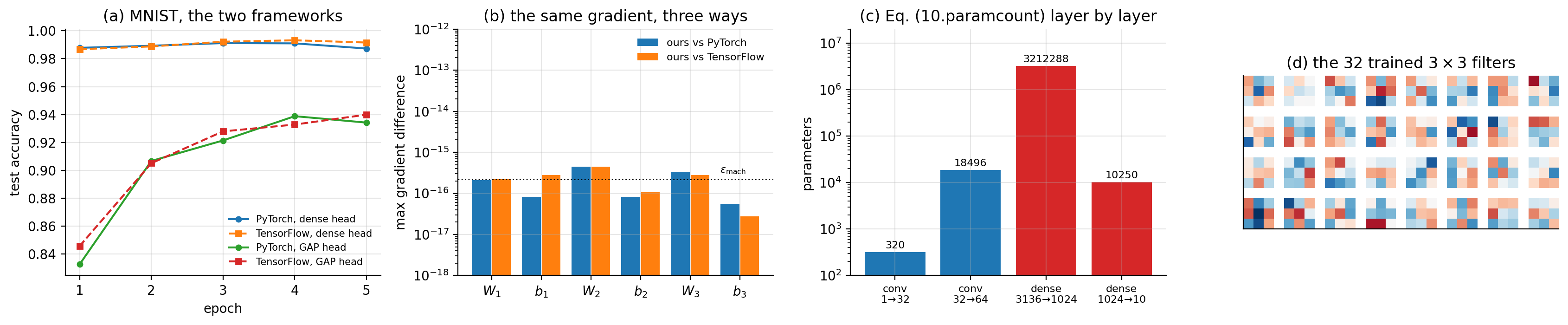
Figure 10.9: (a) Test accuracy against epoch on MNIST for the network of Section The same network in PyTorch and TensorFlow in both frameworks, with the dense head of the listings and with global average pooling in its place; the two frameworks lie on top of one another and the two heads do not. (b) The largest disagreement between our hand-derived gradients, Eqs. (10.26)–(10.28), and the same gradients obtained by automatic differentiation in each framework, against the double-precision unit roundoff. (c) Parameters per layer from Proposition 10.4: the two convolutional layers hold \(0.58\%\) of the network. (d) The thirty-two \(3\times3\) first-layer filters of the trained PyTorch model, on the same colour scale; compare Figure 10.8(c), which shows the same structure emerging in the NumPy network on \(8\times8\) digits.
10.11. Summary and the programs#
A convolutional layer is what remains of a dense layer after we insist that it respect the structure of the data. Locality makes the matrix banded, parameter sharing makes its diagonals constant, and by Theorem 10.2 a banded matrix with constant diagonals is exactly a convolution. The stronger statement is Theorem 10.7: convolution is the only linear map that commutes with translation, so the architecture is not a heuristic but the unique consequence of a symmetry assumption. The parameter count falls from \(\bigO(L^{4})\) per layer to \(K(CF^{2}+1)\), independent of image size.
Backpropagation required no new ideas. The gradients (10.26)–(10.28) are the chain rule applied to Eq. (10.16), and all three are the adjoint of the forward map, which we verified as an inner-product identity to \(10^{-14}\). Max pooling routes the gradient to the argmax and is differentiable almost everywhere.
The experiment of Section Does it actually help? An experiment should be remembered together with the theory. On centred \(8\times8\) digits the convolutional network was not better than a dense network with the same number of parameters, \(0.9656\) against \(0.9670\); on the same digits placed at random offsets it was better by seventeen points with \(2.5\) times fewer parameters. The inductive bias pays exactly when the assumption behind it is true, and not otherwise.
Three structural results were added along the way and each pays off later. Theorem 10.3 says every circulant matrix is diagonalised by the same Fourier basis, so a convolutional layer multiplies each frequency by a learned number; the alternation between a map diagonal in frequency and a non-linearity diagonal in space is where the expressive power lives. Proposition 10.11 shows that dilation buys an exponentially growing receptive field at linear parameter cost and no loss of resolution – five layers rather than thirty-one for \(R=63\). And Proposition 10.12 identifies the backward pass as the transposed convolution, with the output size (10.29) that every generator in Part IV is designed around, and explains the checkerboard artefacts that follow from choosing \(F\) not a multiple of \(S\).
The comparison against the libraries in Section Do the three implementations agree? is the strongest verification in the chapter. Pushing one set of weights into our NumPy code, PyTorch and TensorFlow, the forward passes agree to \(1.8\times10^{-15}\) and every gradient to \(4.4\times10^{-16}\) – unit roundoff. The finite-difference check of Section Verifying the implementation compared our gradient against our own forward pass and would have passed had both been wrong in the same way; this one compares against two independent implementations. Trained on the full MNIST set the same architecture reaches \(0.9873\) in PyTorch and \(0.9916\) in TensorFlow after five epochs, a difference the size of the epoch-to-epoch variation of either.
Two practical warnings are worth carrying forward. A ReLU and max-pool network cannot be gradient-checked naively, because the function is piecewise linear and a central difference straddles the kinks; check on a smooth surrogate instead. And in a classical architecture the convolutional layers hold a tiny fraction of the parameters – \(0.58\%\), measured – while the first dense layer holds \(99.1\%\), so that is where the memory and the overfitting live. Replacing it by global average pooling cuts the parameter count by a factor of \(167\) and costs about five points of accuracy in five epochs, which is a real trade rather than a free lunch.
The programs are in the directory
doc/BookML/BookPrograms/chapter10_convolutional_networks.
Every listing above appears there as a numbered file, and two self-contained modules run start to finish and reproduce the numbers quoted in the text:
cnn.py– im2col, the convolution and pooling layers with their gradients, the network of Eq. (10.32), He initialisation and Adam.verify_cnn.py– all four checks of Section Verifying the implementation: the naive-loop comparison, the adjoint identity, the finite-difference gradient checks including the ReLU failure and its smooth-surrogate resolution, the Toeplitz and doubly block Toeplitz reconstructions, and the equivariance tests.run_digits.pyandrun_shift.py– the two blocks of Table 10.1.cross_check.py– the three-way comparison of Section Do the three implementations agree?: one set of weights pushed into our code, PyTorch and TensorFlow, with the layout conversions written out, and the parameter counts of Section Parameter counts, checked.cnn_torch.pyandcnn_tf.py– the MNIST training of Section Training on MNIST, and what the dense layer is worth in each framework, with the dense and the global-average-pooling heads selectable.mnist_data.py– a loader that reads MNIST from a local.npz, so that the programs run on a machine with no outbound network access.
The figures are generated by ch10_figures.py in
doc/BookML/BookFigures; none is drawn by hand.
10.12. Exercises#
10.12.1. Warm-up exercises#
Convolution arithmetic. Use Proposition 10.4 throughout. (a) An input of \(32\times32\times3\) with \(K=32\) filters of extent \(F=3\), \(S=1\), \(P=0\): what is the output volume and how many parameters does the layer have? (b) Repeat with \(P=1\) and explain why this padding is the usual choice. (c) Find all \((F,P)\) with \(S=1\) that preserve the spatial size, and show that \(F\) must be odd. (d) An input of \(28\times28\) with \(F=5\), \(S=3\), \(P=1\): show that the floor in Eq. (10.17) is doing real work, and identify which input rows are never seen.
Polynomial multiplication. Multiply \(p(t)=2-t+3t^{2}\) by \(s(t)=1+4t-2t^{2}+5t^{3}\) by hand, then reproduce the coefficients with \verb!np.convolve! and with the Toeplitz matrix of Eq. (10.8). Verify that the matrix satisfies Definition 10.1, and confirm the commutativity \(\bm{T}_\alpha\bm{\beta}=\bm{T}_\beta\bm{\alpha}\).
Convolution or cross-correlation. Take a \(5\times5\) input and a non-symmetric \(3\times3\) kernel. Compute both Eq. (10.14) and Eq. (10.15) and show that the results differ but are related by a \(180^{\circ}\) rotation of the kernel. Then argue why this makes no difference to a trained network, and construct a case where it does.
Receptive field. (a) Using Eq. (10.22), find the receptive field of a stack of five \(3\times3\) convolutions with \(S=1\). (b) Insert a \(2\times2\) pooling layer after every second convolution and recompute. (c) Show that two \(3\times3\) layers have the same receptive field as one \(5\times5\) layer but fewer parameters, and state the other advantage.
Equivariance by hand. Prove the forward direction of Theorem 10.7 for the two-dimensional case. Then show by explicit counterexample that a dense layer is not equivariant, and that max pooling with \(F=S=2\) is invariant to shifts of one pixel only when the argmax does not cross a window boundary.
The adjoint. Show that \(\mathrm{col2im}\) as implemented is the adjoint of \(\mathrm{im2col}\), by verifying \(\langle\mathcal{A}\bm{x},\bm{y}\rangle=\langle\bm{x},\mathcal{A}^{*}\bm{y}\rangle\) for random \(\bm{x},\bm{y}\) and several \((F,S,P)\). Explain why \verb!np.add.at! rather than plain assignment is essential when \(S<F\).
The convolution theorem. (a) Prove Theorem 10.3 for \(n=4\) by writing out the \(4\times4\) circulant matrix and the four Fourier modes explicitly. (b) Verify Eq. (10.11) numerically with \verb!np.fft!, for a random kernel and input, and confirm that the error is at rounding level. (c) Time a direct convolution against the FFT route as a function of the kernel length \(F\) at fixed \(n=4096\), and find the crossover. (d) A convolutional layer multiplies each Fourier mode by one number. What does that say about the function a single convolutional layer with no activation can represent, however many filters it has?
Dilation. (a) Derive Eq. (10.25) from Eq. (10.22). (b) How many layers of \(3\times3\) filters are needed for a receptive field of \(255\) with \(D_\ell=2^{\ell-1}\), and how many without dilation? (c) Dilated convolutions can miss pixels – the “gridding” artefact. For two stacked layers with \(F=3\) and \(D=2\) in both, find an input pixel that no output depends on, and suggest a schedule of rates that avoids it.
Transposed convolution. (a) Verify Eq. (10.29) for \(F=4\), \(S=2\), \(P=1\) and \(H_2=7\), and check the answer against \verb!nn.ConvTranspose2d!. (b) Build the matrix \(\bm{W}'\) of Eq. (10.19) for a small example and confirm that \(\bm{W}'^{\top}\) is what the library computes. (c) Show that with \(F=3\), \(S=2\) the output pixels are produced from either one or two input pixels depending on parity, and that \(F=4\), \(S=2\) makes the count uniform. This is the checkerboard artefact.
Reproducing the three-way check. Take the small network of Section Do the three implementations agree? and reconstruct the weight conversions yourself: our \((K,C,F,F)\) into Keras’s \((F,F,C,K)\), and the flatten permutation between \((K,H,W)\) and \((H,W,K)\) ordering. Then deliberately omit the flatten permutation and report what happens to the forward pass, to the gradients, and to the training curve. Which of the three would have caught the mistake?
10.12.2. Project-style exercise: a convolutional network from scratch#
Part a: the layers. Implement \verb!im2col!, \verb!col2im!, the convolution forward and backward passes and max pooling. Verify each against the explicit loop form of Eq. (10.16) for at least four combinations of stride and padding, and verify the adjoint identity.
Part b: gradients. Gradient-check the complete network against central differences. You should find that the check fails for at least one parameter array; diagnose it, and show that replacing ReLU and max pooling by smooth surrogates repairs it. State what this implies about testing any piecewise-linear model.
Part c: the structural claims. Reconstruct the matrix \(\bm{W}'\) of Eq. (10.19) column by column from your own \verb!conv_forward!. Confirm the number of non-zero entries and the number of distinct values, and display its doubly block Toeplitz structure. Measure the equivariance error for \(S=1\) and \(S=2\) over a range of shifts and compare with Proposition 10.8.
Part d: the experiment. Reproduce Table 10.1: the centred and the translated digits, CNN and dense, matched parameter counts, at least five seeds. Report the spread honestly and say whether the difference in the upper block is significant.
Part e: what breaks it. Equivariance is to translation. Rotate or rescale the digits instead and repeat the comparison. Does the convolutional network retain its advantage? Explain your answer with reference to Theorem 10.7, and describe what would have to change in the architecture to obtain equivariance to rotation.
Part f: against a library. Rebuild the same architecture in PyTorch or TensorFlow and compare accuracy, runtime and memory with your NumPy version on the same data. Then verify that the library agrees with your implementation numerically: feed both the same weights and the same input and compare the forward and backward passes to machine precision. Any discrepancy is a bug in one of them, and finding out which is the point of the exercise.
Part g: scaling. Using Eqs. (10.1) and (10.18), tabulate the parameter count of a dense and a convolutional first layer for images of side \(32\), \(128\), \(512\) and \(2048\). Then measure how the runtime of your own \verb!conv_forward! scales with image side and with filter size, and compare against the operation counts \(\bigO(NKCF^{2}H_2W_2)\). Where does im2col memory become the binding constraint?