
3. Chapter 3: Linear Regression#
Linear regression is the oldest method in this book and, for the purposes of learning the subject, by far the most valuable. It is the only family of models for which every question we shall want to ask of a machine learning method can be answered in closed form: we can write down the optimal parameters, their bias, their variance, their sensitivity to the data, and the exact effect of regularisation, all with the linear algebra of Chapter 1 and the statistics of Chapter 2. Everything that follows in this book – logistic regression, neural networks, tree ensembles – introduces complications that make one or more of these questions intractable. It is worth understanding thoroughly the one case where nothing is hidden.
The chapter proceeds from the general to the particular. We set up the linear model and derive ordinary least squares from three independent starting points – as an optimisation problem, as an orthogonal projection, and as maximum likelihood under Gaussian noise – and then examine the statistical properties of the resulting estimator. We then add regularisation, first the \(2\)-norm penalty that gives Ridge regression and then the \(1\)-norm penalty that gives the Lasso, and show that the two behave very differently for reasons that are entirely geometric. A Bayesian reading unifies all three as maximum-a-posteriori estimates under different priors. We close with the practical questions of scaling and the intercept, with the procedure by which the penalty is actually chosen – cross-validation, done properly, and compared with the bootstrap – and with a complete worked analysis of the Franke function.
3.1. The regression problem#
We are given \(n\) observations of \(p\) features, collected in the design matrix \(\bm{X}\in\mathbb{R}^{n\times p}\) of Eq. (1.1), together with \(n\) targets \(\bm{y}\in\mathbb{R}^{n}\). We assume the targets are generated by
with \(f\) an unknown function and \(\bm{\varepsilon}\) independent noise, exactly as in Eq. (2.49). Our task is to construct an approximation \(\tilde{\bm{y}}\) to \(f\) from the data.
What makes a model good?. It is worth being explicit, because the answer is not obvious and the obvious answer is wrong. A good model is not one that reproduces the training data accurately; by Section Training error, test error and generalisation that is trivial to achieve and tells us nothing. A good model is one that predicts well on data it has not seen, and by the decomposition (2.52) its expected error on such data is the sum of a squared bias, a variance and an irreducible noise term. The entire content of this chapter is the management of the first two.
Our approach throughout is frequentist: we treat the parameters \(\bm{\theta}\) as fixed but unknown quantities and the data as random, so that statements about uncertainty are statements about what would happen if the data were collected again. Section A Bayesian reading shows what the same methods look like from a Bayesian viewpoint, in which the parameters are random and the data are fixed, and the two readings turn out to produce identical formulae from different premises.
3.2. The linear model and the design matrix#
The model we shall study throughout is linear in the parameters,
with \(\bm{X}_{i,\ast}\) the \(i\)th row. The word linear refers to the parameters and not to the features, and this distinction is the source of most of the method’s usefulness. Nothing prevents the columns of \(\bm{X}\) from being non-linear functions of some underlying variable. If we have a single input \(x\) and choose
then Eq. (3.2) is a polynomial fit of degree \(p-1\), and it remains a linear regression problem. More generally, replacing \(x\) by any set of basis functions \(\phi_j(x)\) – polynomials, splines, Fourier modes, radial basis functions – gives
which is a basis expansion, and every method of this chapter applies verbatim. The matrix (3.3) is the Vandermonde matrix whose appalling conditioning we met in Section Vector and matrix norms; the choice of basis is therefore not only a modelling decision but a numerical one, and an orthogonal polynomial basis is very much better behaved than the monomials.
The first column of ones deserves a name. Its coefficient \(\theta_0\) is the intercept, the predicted value when every other feature vanishes, and it will require separate treatment when we come to regularisation in Section Scaling, centring and the intercept.
Complexity. The number of columns \(p\) measures the flexibility of the model, and it is the knob we turn when tracing out the bias-variance curve of Section The bias-variance tradeoff. For a polynomial in one variable of degree \(d\) we have \(p=d+1\); for a polynomial of degree \(d\) in two variables \(x\) and \(y\), which is the case we shall need for the Franke function, every monomial \(x^{a}y^{b}\) with \(a+b\le d\) appears and
A fifth-order fit in two variables therefore has \(21\) parameters, and a tenth-order fit has \(66\): complexity grows quickly, and with it the danger that \(p\) approaches or exceeds \(n\).
import numpy as np

def design_matrix_2d(x, y, degree):
    """Design matrix for a two-dimensional polynomial of the given degree.

    Columns are the monomials x^a y^b with a + b <= degree, ordered by
    total degree.  The first column is the intercept.
    """
    x, y = np.ravel(x), np.ravel(y)
    columns = []
    for total in range(degree + 1):
        for b in range(total + 1):
            columns.append(x**(total - b) * y**b)
    return np.column_stack(columns)


# A degree-5 fit in two variables has (5+1)(5+2)/2 = 21 parameters
X = design_matrix_2d(np.random.rand(100), np.random.rand(100), degree=5)
print(X.shape)
3.3. Ordinary least squares#
The cost function of ordinary least squares (OLS) is the mean squared error of Eq. (1.34),
and the optimisation problem is
We derived the solution in Section The mean squared error and its derivative: setting the gradient (1.38) to zero gives the normal equations
with Hessian \(2\bm{X}^{T}\bm{X}/n\), positive semi-definite by Eq. (1.44), so that the problem is convex and the stationary point is a global minimum – unique precisely when the columns of \(\bm{X}\) are linearly independent.
The geometric reading. Equation (3.8) has an interpretation which is worth as much as the algebra. The vector \(\bm{X}\bm{\theta}\) ranges over the column space of \(\bm{X}\) as \(\bm{\theta}\) ranges over \(\mathbb{R}^{p}\), so Eq. (3.7) asks for the point of that subspace closest to \(\bm{y}\). By Section Orthonormal bases and projections the answer is the orthogonal projection of \(\bm{y}\) onto the column space, and the projector is the hat matrix
which is symmetric and idempotent as required by Eq. (1.9), with \(\mathrm{Tr}(\bm{H})=p\) by Eq. (1.10). Equivalently, the normal equations (3.8) may be read as \(\bm{X}^{T}(\bm{y}-\bm{X}\bm{\theta})=\bm{0}\): at the optimum the residual is orthogonal to every column of the design matrix. The fit has extracted from \(\bm{y}\) everything that lies in the span of the features and left the rest untouched.
Optimality without calculus. Setting a gradient to zero shows that \(\hat{\bm{\theta}}\) is a stationary point, and convexity then makes it a minimum. There is a shorter route which gives more, and which will be reused for Ridge regression, for the Lasso and for the kernel methods of Section Kernel methods: regression without coordinates.
Proposition 3.1 (Least-squares decomposition)
Let \(\hat{\bm{\theta}}\) be any solution of Eq. (3.8), the normal equations. Then for every \(\bm{\theta}\) in \(\mathbb{R}^{p}\),
Proof
Write \(\bm{y}-\bm{X}\bm{\theta} =(\bm{y}-\bm{X}\hat{\bm{\theta}})-\bm{X}(\bm{\theta}-\hat{\bm{\theta}})\) and expand the square:
The middle term vanishes identically, because \(\bm{X}^{T}(\bm{y}-\bm{X}\hat{\bm{\theta}})=\bm{0}\) is precisely the normal equations. The last term is a quadratic form in the positive semi-definite matrix \(\bm{X}^{T}\bm{X}\) and is therefore non-negative. \qed
Three consequences follow at once, and it is worth being explicit about them because each is used later.
First, \(\hat{\bm{\theta}}\) is a global minimiser, with no appeal to convexity or to second derivatives: the second term of Eq. (3.10) is non-negative and vanishes at \(\bm{\theta}=\hat{\bm{\theta}}\). Second, the minimiser is unique if and only if \(\bm{X}^{T}\bm{X}\) is positive definite, that is if and only if the columns of \(\bm{X}\) are linearly independent; otherwise the second term vanishes on the whole null space of \(\bm{X}\) and every point of an affine subspace attains the minimum. Note carefully what remains unique in that case: the fit \(\bm{X}\hat{\bm{\theta}}\), since two minimisers differ by a vector in the null space of \(\bm{X}\). This distinction between a non-unique parameter and a unique prediction will return for the Lasso in Proposition 3.9. Third, the cost rises away from the optimum at a rate set by the eigenvalues of \(\bm{X}^{T}\bm{X}\): sharply in the directions of large singular value and almost not at all in the directions of small ones. That is the same statement as the variance formula of Section Statistical properties of the least-squares estimator and as the convergence rate of Chapter 4; a flat valley is a direction that the data do not determine, and all three chapters are describing it in their own vocabulary.
How to compute it. Equation (3.8) is a statement about \(\hat{\bm{\theta}}\) and not an instruction to a computer. Forming \(\bm{X}^{T}\bm{X}\) squares the condition number, Eq. (1.118), and for a polynomial design matrix of even modest degree this destroys most of the available precision. The stable routes are the QR decomposition (1.12) or the singular value decomposition, and through the latter the solution is the pseudoinverse of Eq. (1.121),
which additionally handles the rank-deficient case, returning the minimum-norm solution when \(p>n\) or when features are exactly collinear. Equation (3.11) will be our main analytical tool in this chapter: almost everything that follows is a statement about what happens to the factors \(1/\sigma_i\).
import numpy as np

def ols(X, y):
    """Ordinary least squares through the SVD -- never the normal equations."""
    U, s, Vt = np.linalg.svd(X, full_matrices=False)
    return Vt.T @ (U.T @ y / s)


def ols_normal_equations(X, y):
    """The textbook formula.  Shown for comparison; do not use it."""
    return np.linalg.pinv(X.T @ X) @ X.T @ y
Machine learning connection
The two functions above agree to
machine precision on a well-conditioned design matrix and can disagree in the
first significant digit on a badly conditioned one. A simple experiment makes
the point: fit a polynomial of degree twelve to a hundred points on \([0,1]\)
using both. The condition number of the Vandermonde
matrix (3.3) is then of order \(10^{8}\), that of
\(\bm{X}^{T}\bm{X}\) of order \(10^{16}\), and the second function returns
coefficients with no correct digits at all while the first is still accurate.
This is the practical content of Section The singular value decomposition, and it is why
numpy.linalg.lstsq exists.
3.4. Weighted least squares and the \(\chi^2\) function#
The cost function (3.6) treats every observation as equally reliable. In the physical sciences this is rarely true: a measurement is normally accompanied by an error estimate, and points known to ten per cent should not constrain the fit as strongly as points known to one per cent. Introducing the standard deviation \(\sigma_i\) of measurement \(i\), we define the \(\chi^2\) function
where \(\bm{\Sigma}\) is the diagonal matrix with entries \(\sigma_i\). Each residual is measured in units of its own uncertainty, so that the terms of the sum are comparable.
Minimising Eq. (3.12) is the same calculation as before with a weight inserted. Differentiating with the machinery of Section Four worked examples gives
and hence the weighted normal equations
Defining \(\bm{A}=\bm{\Sigma}^{-1}\bm{X}\) and \(\bm{b}=\bm{\Sigma}^{-1}\bm{y}\) turns Eq. (3.14) into the ordinary solution (3.8) for \(\bm{A}\) and \(\bm{b}\): weighted least squares is unweighted least squares on rescaled data. Setting all \(\sigma_i\) equal recovers OLS, which shows what the unweighted method silently assumes – that the noise is homoscedastic, of the same variance everywhere. When it is not, OLS remains unbiased but is no longer the estimator of smallest variance, and Eq. (3.14) is.
Correlated noise: generalised least squares. The same rescaling handles the general case in which the noise has an arbitrary covariance matrix, \(\var(\bm{\varepsilon})=\bm{\Omega}\), symmetric and positive definite. Factor it as \(\bm{\Omega}=\bm{L}\bm{L}^{T}\) by the Cholesky decomposition of Section LU and Cholesky decompositions and multiply the model \(\bm{y}=\bm{X}\bm{\theta}+\bm{\varepsilon}\) by \(\bm{L}^{-1}\): the transformed noise \(\bm{L}^{-1}\bm{\varepsilon}\) has covariance \(\bm{L}^{-1}\bm{\Omega}\bm{L}^{-T}=\bm{I}\), so it is homoscedastic and uncorrelated, and OLS on the whitened data \(\bm{A}=\bm{L}^{-1}\bm{X}\), \(\bm{b}=\bm{L}^{-1}\bm{y}\) gives
the second statement following from \(\var(\bm{A}^{+}\bm{b}) =\bm{A}^{+}\bm{I}(\bm{A}^{+})^{T}=(\bm{A}^{T}\bm{A})^{-1}\). Weighted least squares is the diagonal case \(\bm{\Omega}=\bm{\Sigma}^{2}\), and its variance is \((\bm{X}^{T}\bm{\Sigma}^{-2}\bm{X})^{-1}\). That this is the smallest variance attainable by any linear unbiased estimator is the Gauss-Markov theorem of Section Statistical properties of the least-squares estimator applied to the whitened problem, for which its hypotheses hold exactly.
The value of \(\chi^{2}\) at the minimum. A physicist reports not only the fitted parameters but the minimum value of \(\chi^{2}\), and reads it as a test of the model. The reason is a small calculation. Write \(\bm{b}=\bm{A}\bm{\theta}+\bm{\eta}\) for the whitened data, with \(\var(\bm{\eta})=\bm{I}\), and let \(\bm{H}_A=\bm{A}(\bm{A}^{T}\bm{A})^{-1}\bm{A}^{T}\) be its hat matrix. The whitened residual is \(\bm{b}-\bm{A}\hat{\bm{\theta}}=(\bm{I}-\bm{H}_A)\bm{b} =(\bm{I}-\bm{H}_A)\bm{\eta}\), because \((\bm{I}-\bm{H}_A)\bm{A}=\bm{0}\) removes the model exactly. Then, using \(\mathbb{E}[\bm{\eta}^{T}\bm{M}\bm{\eta}] =\mathrm{Tr}(\bm{M}\,\var(\bm{\eta}))=\mathrm{Tr}(\bm{M})\) for any fixed matrix \(\bm{M}\) and the projector properties (1.9) and (1.10),
If the model is right and the \(\sigma_i\) are right, the sum of squared standardised residuals is on average the number of data points minus the number of fitted parameters, so the reduced \(\chi^{2}\), \(n\chi^{2}_{\min}/(n-p)\), should be close to one. A value well above one says that the model does not describe the data at the stated precision; a value well below one says that the error bars were overestimated. Under Gaussian noise \(n\chi^{2}_{\min}\) has exactly the \(\chi^{2}\) distribution with \(n-p\) degrees of freedom, which Proposition 3.3 will establish, and the statement can then be made quantitative. A short simulation confirms Eq. (3.16) and the variance in Eq. (3.15):
import numpy as np

rng = np.random.default_rng(2024)
n, p = 50, 3
x = np.linspace(0, 1, n)
X = np.c_[np.ones(n), x, x**2]
theta_true = np.array([1.0, -2.0, 3.0])
sigmas = 0.05 + 0.3 * x                    # heteroscedastic: error grows with x

chi2_min, theta_wls, theta_ols = [], [], []
for trial in range(20000):
    y = X @ theta_true + sigmas * rng.normal(size=n)
    A, b = X / sigmas[:, None], y / sigmas   # whitened problem, Eq. (3.chisquared)
    th = np.linalg.lstsq(A, b, rcond=None)[0]
    chi2_min.append(np.sum((b - A @ th)**2) / n)
    theta_wls.append(th)
    theta_ols.append(np.linalg.lstsq(X, y, rcond=None)[0])

print("mean of n*chi2_min:", n * np.mean(chi2_min), "   n - p =", n - p)
print("variance of WLS  :", np.var(theta_wls, axis=0))
print("predicted, (X^T S^-2 X)^-1:", np.diag(np.linalg.inv(X.T @ (X / sigmas[:, None]**2))))
print("variance of OLS  :", np.var(theta_ols, axis=0))
mean of n*chi2_min: 47.07    n - p = 47
variance of WLS  : [0.00090 0.05706 0.09014]
predicted, (X^T S^-2 X)^-1: [0.00088 0.05677 0.08989]
variance of OLS  : [0.00244 0.13275 0.17519]
The unweighted estimator is unbiased here too, but its variance is between two and three times larger: it lets the noisy points at large \(x\) pull the fit as hard as the precise ones at small \(x\).
3.5. Measures of quality#
Before comparing models we must agree on how to score them. The mean squared error
is the quantity we minimise and the natural quantity to report, but it carries the squared units of the target and its numerical value therefore says nothing on its own. The coefficient of determination
is dimensionless and compares the model against the best constant prediction: \(R^{2}=1\) is a perfect fit, \(R^{2}=0\) means the model does no better than predicting the mean, and negative values – entirely possible on test data – mean it does worse. Note that the denominator is \(n\) times the sample variance of \(\bm{y}\), so that \(R^{2}\) is one minus the fraction of variance left unexplained.
Where \(R^{2}\) comes from. The definition (3.18) looks like a convention, but for a least-squares fit with an intercept it is forced by geometry, and the derivation explains both its range and its most abused property. Write \(\bm{e}=\bm{y}-\tilde{\bm{y}}=(\bm{I}-\bm{H})\bm{y}\) for the residual. Since \(\bm{H}\) is an orthogonal projector, \(\tilde{\bm{y}}=\bm{H}\bm{y}\) and \(\bm{e}\) are orthogonal and Pythagoras gives
Now suppose the design matrix contains the constant column \(\bm{1}\), as it does whenever an intercept is fitted. The normal equations \(\bm{X}^{T}\bm{e}=\bm{0}\) then include the row \(\bm{1}^{T}\bm{e}=0\): the residuals sum to zero, so \(\bar{\tilde{y}}=\bar{y}\), and the vector \(\bm{y}-\bar{y}\bm{1}\) decomposes as \((\tilde{\bm{y}}-\bar{y}\bm{1})+\bm{e}\) with the two parts again orthogonal, because \(\bm{e}\perp\tilde{\bm{y}}\) and \(\bm{e}\perp\bm{1}\). Applying Pythagoras once more,
the analysis-of-variance identity: the total sum of squares splits exactly into a part explained by the fit and a residual part. Dividing by the left-hand side,
so on the training data \(R^{2}\) is the squared cosine of the angle between the centred targets and the centred fit, and lies in \([0,1]\). Both halves of that statement fail off the training set: for test data the residuals do not sum to zero and are not orthogonal to the fit, the identity (3.20) breaks, and \(R^{2}\) can be negative.
The identity also proves the warning below. Let \(\bm{X}'=[\bm{X}\;\bm{z}]\) be the design matrix with one further column. Every \(\bm{\theta}\) available to \(\bm{X}\) is available to \(\bm{X}'\) with a zero in the last place, so \(\min_{\bm{\theta}'}\|\bm{y}-\bm{X}'\bm{\theta}'\|^{2} \le\min_{\bm{\theta}}\|\bm{y}-\bm{X}\bm{\theta}\|^{2}\): the training RSS can only fall when a column is added, and by Eq. (3.21) the training \(R^{2}\) can only rise. When \(p=n\) the column space is all of \(\mathbb{R}^{n}\), \(\bm{H}=\bm{I}\), the RSS is zero and \(R^{2}=1\) whatever the columns contain. The adjusted coefficient
replaces the two sums of squares by unbiased variance estimates – the divisor \(n-p\) will be justified in Proposition 3.2 – and can decrease when a useless column is added, but it is a palliative and not a cure: only data the model has not seen measure what we actually care about.
Two further measures appear in the sources of this book. The mean absolute error
is the \(1\)-norm counterpart of Eq. (3.17) and is far less sensitive to outliers, for the reason discussed in Section Vector and matrix norms: squaring gives a point at ten standard deviations a hundred times the weight of one at a single standard deviation, whereas the absolute value gives it ten times. The relative error \(|y_i-\tilde{y}_i|/|y_i|\) is natural when the targets span orders of magnitude, and dangerous when any of them is near zero.
import numpy as np

def mse(y, y_tilde):
    return np.mean((y - y_tilde)**2)

def r2(y, y_tilde):
    return 1.0 - np.sum((y - y_tilde)**2) / np.sum((y - np.mean(y))**2)

def mae(y, y_tilde):
    return np.mean(np.abs(y - y_tilde))
A warning is in order. All three are meaningful only on data held out from fitting. Computed on the training set, \(R^{2}\) increases monotonically as columns are added to \(\bm{X}\) and reaches unity when \(p=n\), whatever those columns contain – including pure noise. Every number reported in this chapter is a test quantity unless we say otherwise.
3.6. Deriving least squares from a probability distribution#
So far the squared-error cost (3.6) has been an assumption. We now show that it follows from a statement about the noise, which both explains where it comes from and makes clear when it is the wrong choice.
Under the model (3.1), and given that the entries of the design matrix are not stochastic, the target \(y_i\) is Gaussian with mean \(\bm{X}_{i,\ast}\bm{\theta}\) and variance \(\sigma^{2}\),
which is Eq. (2.39) written out in full. Reading Eq. (3.24) as a function of the parameters rather than of the data gives the likelihood of observing \(y_i\) given \(\bm{\theta}\), and since the observations are independent and identically distributed the likelihood of the whole data set \(\bm{D}\) is the product
where \(\bm{D}\) denotes the domain of events, inputs and targets together; in the one-dimensional case \(\bm{D}=[(x_0,y_0),(x_1,y_1),\dots,(x_{n-1},y_{n-1})]\).
Maximum likelihood estimation chooses the parameters making the observed data most probable, that is maximising Eq. (3.25). Differentiating a product of \(n\) terms is awkward and numerically hazardous, since the product of many small numbers underflows. Because the logarithm is monotonically increasing, maximising the likelihood is equivalent to maximising its logarithm, and we prefer to minimise the negative of that:
Inserting Eq. (3.24) the sum evaluates to
The first term does not involve \(\bm{\theta}\), and the second is the least-squares cost (3.6) up to a positive constant. Differentiating therefore returns \(\bm{X}^{T}(\bm{y}-\bm{X}\bm{\theta})=\bm{0}\) and
once more.
The noise variance by maximum likelihood. The likelihood (3.27) also depends on \(\sigma^{2}\), and maximising over it as well is instructive. Differentiating Eq. (3.27) with respect to \(\sigma^{2}\),
the training mean squared error. This estimator is biased: it divides by \(n\) where Proposition 3.2 will show that \(n-p\) is required, because the residuals of a fitted model are systematically smaller than the noise that produced them. Maximum likelihood is a principle for choosing estimators, not a guarantee that they are unbiased, and this is the simplest example of the difference.
Fisher information and the Cram’er-Rao bound.
The Gaussian likelihood delivers one more result, and it puts the variance formula that Section Statistical properties of the least-squares estimator will use into a wider frame. The Fisher information is the expected negative Hessian of the log-likelihood with respect to the parameters,
where the second equality uses \(C=-\log p\) and the third differentiates Eq. (3.27) twice, as in Section The Hessian matrix; the expectation is trivial because the Hessian does not depend on the data. It measures how sharply the data pin down the parameters – how curved the log-likelihood is at its peak. The Cram’er-Rao inequality, proved in any text on mathematical statistics, states that every unbiased estimator \(\tilde{\bm{\theta}}\) of \(\bm{\theta}\) satisfies
in the sense that the difference is positive semi-definite. Comparing with the variance of the least-squares estimator, Eq. (3.32) below, the bound is attained: under Gaussian noise OLS is efficient, of minimum variance among all unbiased estimators, linear or not. This is stronger than the Gauss-Markov theorem, which restricts the competition to linear estimators but in return needs no Gaussian assumption; the two results bracket the same estimator from different sides.
Machine learning connection
Equation (3.27) says that least squares is maximum likelihood for Gaussian noise, and the converse statement is the useful one: a different noise model gives a different loss function. Laplace-distributed noise gives the mean absolute error (3.23); Bernoulli-distributed targets give the cross-entropy loss of logistic regression; Poisson counts give the Poisson deviance. When we later write down a loss function for a neural network we are, whether or not we say so, making an assumption about the distribution of the residuals. Choosing the squared error for data with heavy-tailed noise is not a matter of taste but an error, and it is why a handful of outliers can dominate a least-squares fit.
3.7. Statistical properties of the least-squares estimator#
Because \(\hat{\bm{\theta}}\) is a function of the random targets, it is itself a random variable, and Section The statistics of the least-squares estimator established its first two moments:
The estimator is unbiased provided the linear model is correct, and its covariance matrix is the inverse Hessian scaled by the noise variance. Since \(\sigma^{2}\) is unknown it is estimated from the residuals,
the divisor \(n-p\) accounting for the \(p\) degrees of freedom consumed by the fit, in the manner of Bessel’s correction (2.28). The standard error of coefficient \(j\) is then \(\hat{\sigma}\sqrt{[(\bm{X}^{T}\bm{X})^{-1}]_{jj}}\), from which a confidence interval follows,
with \(t\) the appropriate quantile of Student’s distribution, which for \(n-p\) large is simply the Gaussian quantile, \(1.96\) for \(95\%\).
Each of these statements is used constantly and each deserves a proof; the proofs are short and they introduce the residual projector \(\bm{I}-\bm{H}\), which is the key to everything in this section. Throughout, \(\bm{y}=\bm{X}\bm{\theta}+\bm{\varepsilon}\) with \(\mathbb{E}[\bm{\varepsilon}] =\bm{0}\) and \(\var(\bm{\varepsilon})=\sigma^{2}\bm{I}\), and \(\bm{X}\) has full column rank.
Proposition 3.2 (The residual variance estimator is unbiased)
The residual vector is \(\bm{e}=\bm{y}-\bm{X}\hat{\bm{\theta}} =(\bm{I}-\bm{H})\bm{\varepsilon}\), and \(\mathbb{E}\big[\|\bm{e}\|_2^{2}\big]=(n-p)\sigma^{2}\). Hence \(\hat{\sigma}^{2}\) of Eq. (3.33) satisfies \(\mathbb{E}[\hat{\sigma}^{2}]=\sigma^{2}\).
Proof
Since \(\bm{H}\bm{X}=\bm{X}\), we have \((\bm{I}-\bm{H})\bm{y} =(\bm{I}-\bm{H})\bm{X}\bm{\theta}+(\bm{I}-\bm{H})\bm{\varepsilon} =(\bm{I}-\bm{H})\bm{\varepsilon}\): the residual projector annihilates the model and sees only the noise. Then, because \(\bm{I}-\bm{H}\) is symmetric and idempotent,
using \(\mathbb{E}[\bm{z}^{T}\bm{M}\bm{z}]=\mathrm{Tr}(\bm{M}\var(\bm{z}))\) for a zero-mean vector \(\bm{z}\) and \(\mathrm{Tr}(\bm{H})=p\) from Eq. (1.10). \qed
The projector \(\bm{I}-\bm{H}\) has \(n-p\) eigenvalues equal to one and \(p\) equal to zero, so the residual lives in an \((n-p)\)-dimensional subspace: that is the precise sense in which the fit “consumes \(p\) degrees of freedom”. Under Gaussian noise the same projector gives the full distribution theory behind the confidence interval (3.34).
Proposition 3.3 (Distribution of the least-squares estimator)
Assume in addition that the noise is Gaussian, \(\bm{\varepsilon}\sim\mathcal{N}(\bm{0},\sigma^{2}\bm{I})\). Then
\(\hat{\bm{\theta}}\sim\mathcal{N}\!\left(\bm{\theta}, \sigma^{2}(\bm{X}^{T}\bm{X})^{-1}\right)\);
\(\hat{\bm{\theta}}\) and the residual \(\bm{e}\) are independent;
\((n-p)\hat{\sigma}^{2}/\sigma^{2}=\|\bm{e}\|_2^{2}/\sigma^{2}\) has the \(\chi^{2}\) distribution with \(n-p\) degrees of freedom;
for each \(j\), the ratio \((\hat{\theta}_j-\theta_j)\big/\big(\hat{\sigma} \sqrt{[(\bm{X}^{T}\bm{X})^{-1}]_{jj}}\big)\) has Student’s \(t\) distribution with \(n-p\) degrees of freedom.
Proof
(i) \(\hat{\bm{\theta}}=\bm{\theta}+(\bm{X}^{T}\bm{X})^{-1}\bm{X}^{T}\bm{\varepsilon}\) is an affine map of a Gaussian vector and hence Gaussian, with the moments of Eq. (3.32). (ii) Both are linear in \(\bm{\varepsilon}\), so joint Gaussianity holds and independence is equivalent to zero cross-covariance:
because \(\bm{X}^{T}\bm{H}=(\bm{H}\bm{X})^{T}=\bm{X}^{T}\). (iii) By the spectral decomposition of Section The spectral decomposition of symmetric matrices, \(\bm{I}-\bm{H}=\bm{Q}\bm{D}\bm{Q}^{T}\) with \(\bm{Q}\) orthogonal and \(\bm{D}\) diagonal with \(n-p\) ones and \(p\) zeros. Put \(\bm{w}=\bm{Q}^{T}\bm{\varepsilon}/\sigma\); an orthogonal map of \(\mathcal{N}(\bm{0},\bm{I})\) is again \(\mathcal{N}(\bm{0},\bm{I})\), so the \(w_k\) are independent standard normals, and \(\|\bm{e}\|_2^{2}/\sigma^{2}=\bm{w}^{T}\bm{D}\bm{w}\) is the sum of \(n-p\) of their squares, which is the definition of \(\chi^{2}_{n-p}\). (iv) By (i), \(z_j=(\hat{\theta}_j-\theta_j)/(\sigma\sqrt{[(\bm{X}^{T}\bm{X})^{-1}]_{jj}})\) is standard normal; by (iii), \(u=(n-p)\hat{\sigma}^{2}/\sigma^{2}\) is \(\chi^{2}_{n-p}\); by (ii) they are independent; and \(z_j/\sqrt{u/(n-p)}\), which is exactly the ratio in (iv), is by definition Student’s \(t\) with \(n-p\) degrees of freedom. \qed
Statement (iv) is the confidence interval (3.34): the interval \(\hat{\theta}_j\pm t_{\alpha/2,n-p}\,\hat{\sigma}\sqrt{[(\bm{X}^{T}\bm{X})^{-1}]_{jj}}\) covers the true \(\theta_j\) with probability exactly \(1-\alpha\), not approximately, and the Student quantile rather than the Gaussian one is what pays for having estimated \(\sigma\) from the same data. Statement (iii) is also the promised justification of the reduced-\(\chi^{2}\) test of Section Weighted least squares and the \(\chi^2\) function. All four statements can be checked by simulation, and the check is worth running once because it also exposes what the confidence interval does not promise – see the last line of the output.
import numpy as np
from scipy import stats

rng = np.random.default_rng(2024)
n, p, sigma = 30, 4, 0.5
x = np.linspace(-1, 1, n)
X = np.vander(x, p, increasing=True)                 # cubic polynomial
theta_true = np.array([1.0, 0.5, -2.0, 1.5])
XtX_inv = np.linalg.inv(X.T @ X)
t_q = stats.t.ppf(0.975, n - p)                      # 2.056 for n-p = 26

s2, covered, joint, train, test = [], [], [], [], []
for trial in range(20000):
    y = X @ theta_true + sigma * rng.normal(size=n)
    theta = XtX_inv @ X.T @ y
    e = y - X @ theta
    s2.append(e @ e / (n - p))                        # Eq. (3.sigmahat)
    se = np.sqrt(s2[-1] * np.diag(XtX_inv))
    inside = np.abs(theta - theta_true) <= t_q * se  # Eq. (3.confint)
    covered.append(inside); joint.append(inside.all())
    train.append(e @ e / n)                           # training MSE
    y_new = X @ theta_true + sigma * rng.normal(size=n)
    test.append(np.mean((y_new - X @ theta)**2))     # fresh targets, same X

print("E[sigma_hat^2] =", np.mean(s2), "  sigma^2 =", sigma**2)
print("coverage per coefficient:", np.mean(covered, axis=0))
print("all four covered at once:", np.mean(joint))
print("E[train MSE] =", np.mean(train), "  sigma^2 (1 - p/n) =", sigma**2 * (1 - p/n))
print("E[test  MSE] =", np.mean(test),  "  sigma^2 (1 + p/n) =", sigma**2 * (1 + p/n))
E[sigma_hat^2] = 0.24999   sigma^2 = 0.25
coverage per coefficient: [0.9499 0.9498 0.9510 0.9492]
all four covered at once: 0.861
E[train MSE] = 0.21666   sigma^2 (1 - p/n) = 0.21667
E[test  MSE] = 0.28420   sigma^2 (1 + p/n) = 0.28333
The first three lines are Propositions 3.2 and 3.3: the variance estimate is unbiased and each interval covers its coefficient \(95\%\) of the time. The probability that all four intervals cover simultaneously is only \(86\%\) – individual confidence statements do not combine into a joint one, and a table of \(p\) separate intervals says less than it appears to. The last two lines are a result we have not yet derived, and it is the quantitative form of the warning in Section Measures of quality.
Why the training error is optimistic.
Suppose the linear model is correct. By Proposition 3.2 the expected training error is
smaller than the noise level, by exactly the fraction of the noise that the fit has absorbed. Now draw fresh targets \(\bm{y}'=\bm{X}\bm{\theta}+\bm{\varepsilon}'\) at the same inputs, with \(\bm{\varepsilon}'\) independent of \(\bm{\varepsilon}\), and score the fitted model on them. Since \(\bm{y}'-\bm{X}\hat{\bm{\theta}} =\bm{\varepsilon}'-\bm{H}\bm{\varepsilon}\) and the two terms are independent with zero mean,
The difference,
is the amount by which the training error flatters every least-squares fit, and it grows linearly with the number of parameters. A model that adds columns will always look better in training and, once the added columns stop carrying signal, will look worse in test by exactly this margin: that is the bias-variance curve of Section The bias-variance tradeoff for the case in which the bias is already zero, and the variance term is \(p\sigma^{2}/n\). Adding \(2p\hat{\sigma}^{2}/n\) to the training error to correct for it is Mallows’ \(C_p\) statistic, and the same correction with \(\hat{\sigma}^{2}\) replaced by the likelihood is Akaike’s information criterion; both are attempts to estimate the test error from training quantities. Cross-validation, to which we now turn, estimates it directly.
Leave-one-out cross-validation in closed form.
The most thorough version of the cross-validation of Section Cross-validation is leave-one-out: fit \(n\) times, each time omitting one observation, and predict the omitted point. For linear regression it need not be done \(n\) times, and the derivation is a small classic. Let \(\bm{x}_i^{T}\) be row \(i\) of \(\bm{X}\), let \(\hat{\bm{\theta}}_{(-i)}\) be the estimator without observation \(i\), and let \(h_{ii}=\bm{x}_i^{T} (\bm{X}^{T}\bm{X})^{-1}\bm{x}_i\) be the \(i\)th diagonal element of the hat matrix, the leverage of point \(i\). Removing a row changes \(\bm{X}^{T}\bm{X}\) by a rank-one term, \(\bm{X}^{T}\bm{X}-\bm{x}_i\bm{x}_i^{T}\), and the Sherman-Morrison formula
– verified by multiplying both sides by \(\bm{M}-\bm{u}\bm{v}^{T}\) – gives the inverse without a new factorisation. Applying it with \(\bm{M}=\bm{X}^{T}\bm{X}\) and \(\bm{u}=\bm{v}=\bm{x}_i\) to \(\hat{\bm{\theta}}_{(-i)}=(\bm{X}^{T}\bm{X}-\bm{x}_i\bm{x}_i^{T})^{-1} (\bm{X}^{T}\bm{y}-\bm{x}_iy_i)\) and simplifying – the exercises at the end of the chapter ask for the algebra – yields
where \(e_i=y_i-\bm{x}_i^{T}\hat{\bm{\theta}}\) is the ordinary residual of the full fit. The leave-one-out prediction error is therefore the ordinary residual inflated by \(1/(1-h_{ii})\): a point with high leverage pulls the fit towards itself, its residual is deceptively small, and Eq. (3.39) undoes exactly that. Summing gives the leave-one-out estimate of the test error from a single fit,
Allen’s PRESS statistic. Nothing in the derivation used the particular form of \(\bm{H}\) beyond \(\tilde{\bm{y}}=\bm{H}\bm{y}\) being linear in \(\bm{y}\), and the same identity holds for any linear smoother \(\tilde{\bm{y}}=\bm{S}\bm{y}\) with \(h_{ii}\) replaced by \(S_{ii}\); in particular for Ridge regression with \(\bm{S}_\lambda=\bm{X}(\bm{X}^{T}\bm{X}+\lambda\bm{I})^{-1}\bm{X}^{T}\), so that the penalty can be chosen by leave-one-out at the price of one fit per candidate \(\lambda\). Replacing each \(S_{ii}\) by their average \(\mathrm{Tr}(\bm{S})/n\) gives the generalised cross-validation criterion
which is invariant under rotations of the data and depends on the design only through the effective degrees of freedom of Section Ridge regression. The following code checks Eq. (3.40) against \(n\) explicit refits, for OLS and for Ridge, and uses it to choose \(\lambda\).
import numpy as np

rng = np.random.default_rng(7)
n = 40
x = np.sort(rng.random(n))
y = np.sin(2 * np.pi * x) + 0.3 * rng.normal(size=n)
X = np.vander(x, 11, increasing=True)                # degree-10 polynomial

def loo_explicit(X, y, lmbda=0.0):
    # leave-one-out by n separate fits
    n, p = X.shape
    errs = np.empty(n)
    for i in range(n):
        keep = np.arange(n) != i
        theta = np.linalg.solve(X[keep].T @ X[keep] + lmbda * np.eye(p),
                                X[keep].T @ y[keep])
        errs[i] = y[i] - X[i] @ theta
    return np.mean(errs**2)

def loo_closed_form(X, y, lmbda=0.0):
    # the same number from one fit, Eq. (3.press)
    n, p = X.shape
    S = X @ np.linalg.solve(X.T @ X + lmbda * np.eye(p), X.T)   # smoother matrix
    e = y - S @ y
    return np.mean((e / (1.0 - np.diag(S)))**2)

def gcv(X, y, lmbda=0.0):
    # generalised cross-validation, Eq. (3.gcv)
    n, p = X.shape
    S = X @ np.linalg.solve(X.T @ X + lmbda * np.eye(p), X.T)
    e = y - S @ y
    return np.mean(e**2) / (1.0 - np.trace(S) / n)**2

for lmbda in [0.0, 1e-4, 1e-2]:
    print(f"lambda = {lmbda:<6}  explicit {loo_explicit(X, y, lmbda):.6f}"
          f"  closed form {loo_closed_form(X, y, lmbda):.6f}"
          f"  GCV {gcv(X, y, lmbda):.6f}")

lambdas = np.logspace(-8, 0, 81)
print("lambda chosen by LOO:", lambdas[np.argmin([loo_closed_form(X, y, l) for l in lambdas])])
print("lambda chosen by GCV:", lambdas[np.argmin([gcv(X, y, l) for l in lambdas])])
lambda = 0.0     explicit 0.107484  closed form 0.107485  GCV 0.108301
lambda = 0.0001  explicit 0.080349  closed form 0.080349  GCV 0.084748
lambda = 0.01    explicit 0.125840  closed form 0.125840  GCV 0.127780
lambda chosen by LOO: 0.0006309573444801943
lambda chosen by GCV: 0.0006309573444801943
The closed form reproduces the forty explicit refits to every printed digit – the difference of one unit in the last place at \(\lambda=0\) is the rounding of the unpenalised solve on a badly conditioned Vandermonde matrix, Section Ordinary least squares – at a fortieth of the cost. Both criteria have a clear interior minimum, at a penalty that lowers the leave-one-out error from \(0.107\) for the unpenalised degree-ten fit to \(0.080\), and here they pick the same \(\lambda\); in general GCV differs a little because averaging the leverages discounts the high-leverage points at the ends of the interval that dominate the leave-one-out sum for a polynomial fit.
Reading the variance through the SVD. Substituting Eq. (1.115) into Eq. (3.32) gives
so the variance along the \(i\)th right singular direction is \(\sigma^{2}/\sigma_i^{2}\). Together with the expansion (3.11) this gives the complete picture of what collinearity does. A direction in feature space along which the data barely vary has a small singular value; the coefficient along it is obtained by dividing by that small number, and its variance is obtained by dividing by its square. The fit becomes an enormous positive coefficient on one feature cancelling an enormous negative one on another, and the pair swings wildly when the data are perturbed. Nothing is wrong with the algebra; the data simply do not determine that combination.
The Gauss-Markov theorem. Among all estimators that are both linear in \(\bm{y}\) and unbiased, OLS has the smallest variance. This is the Gauss-Markov theorem, and it requires only that the noise have zero mean, constant variance and be uncorrelated – not that it be Gaussian. Its proof is a few lines and shows exactly where the competing estimators lose.
Theorem 3.4 (Gauss-Markov)
Let \(\bm{y}=\bm{X}\bm{\theta}+\bm{\varepsilon}\) with \(\mathbb{E}[\bm{\varepsilon}]=\bm{0}\), \(\var(\bm{\varepsilon})=\sigma^{2}\bm{I}\) and \(\bm{X}\) of full column rank. If \(\tilde{\bm{\theta}}=\bm{C}\bm{y}\) is any estimator linear in \(\bm{y}\) with \(\mathbb{E}[\tilde{\bm{\theta}}]=\bm{\theta}\) for every \(\bm{\theta}\), then \(\var(\tilde{\bm{\theta}})-\var(\hat{\bm{\theta}}_{\mathrm{OLS}})\) is positive semi-definite.
Proof
Unbiasedness for every \(\bm{\theta}\) means \(\mathbb{E}[\bm{C}\bm{y}]=\bm{C}\bm{X}\bm{\theta}=\bm{\theta}\) for all \(\bm{\theta}\), hence \(\bm{C}\bm{X}=\bm{I}\). Write \(\bm{C}=(\bm{X}^{T}\bm{X})^{-1}\bm{X}^{T}+\bm{D}\), which defines \(\bm{D}\); then \(\bm{C}\bm{X}=\bm{I}+\bm{D}\bm{X}\), so \(\bm{D}\bm{X}=\bm{0}\). Now
the two cross terms vanishing because \(\bm{D}\bm{X}=\bm{0}\) and \(\bm{X}^{T}\bm{D}^{T}=(\bm{D}\bm{X})^{T}=\bm{0}\). The first term is \(\var(\hat{\bm{\theta}}_{\mathrm{OLS}})\) and the second is a Gram matrix, positive semi-definite, with equality if and only if \(\bm{D}=\bm{0}\). \qed
Every linear unbiased competitor is OLS plus a piece \(\bm{D}\bm{y}\) that averages to zero and only adds variance. The theorem is often quoted as though it settled the matter. It does not, and the reason is Eq. (2.27): the mean squared error counts bias and variance equally, and Gauss-Markov restricts attention to the unbiased estimators only. The moment we admit biased estimators, better ones exist. The rest of this chapter constructs them.
3.8. Ridge regression#
Ridge regression adds a penalty on the squared length of the parameter vector,
with \(\|\bm{\theta}\|_2^{2}=\sum_j\theta_j^{2}\). We derived the solution in Eq. (1.42); dropping the factor \(1/n\) so that \(\lambda\) has its conventional scaling,
with \(\bm{I}\) the \(p\times p\) identity. Ridge regression is therefore ordinary least squares with a modified diagonal – a fact which Section Kernel methods: regression without coordinates will turn into a method that never forms the design matrix at all – and the modification cures the central defect of Eq. (3.8): whatever the rank of \(\bm{X}\), the matrix \(\bm{X}^{T}\bm{X}+\lambda\bm{I}\) has all eigenvalues at least \(\lambda\) and is invertible for every \(\lambda>0\). The estimator exists even when \(p>n\).
The constrained form. Equation (3.43) is the Lagrangian form of a constrained problem: minimising the squared error subject to
for a finite \(t>0\) gives the same solutions, with a one-to-one decreasing correspondence between \(t\) and \(\lambda\). The constraint region is a ball in parameter space, and this geometric picture is what will distinguish Ridge from the Lasso in Section The Lasso.
Shrinkage, through the SVD. The analytical content of Ridge regression is best seen in the singular basis. Section Ridge regression through the singular value decomposition showed that Eq. (3.44) is
to be compared with the OLS expansion (3.11) in which the coefficient was \(1/\sigma_i\). The fitted values follow from Eq. (1.131),
whereas for OLS the same expression holds with every factor replaced by one, \(\tilde{\bm{y}}_{\mathrm{OLS}}=\bm{U}\bm{U}^{T}\bm{y}\), which is the hat matrix (3.9) in the singular basis. Since \(\lambda\ge0\),
so Ridge regression expresses \(\bm{y}\) in the orthonormal basis \(\bm{U}\) and then shrinks each coordinate. Because the singular values are ordered descendingly, the shrinkage is mild for the leading directions and severe for the trailing ones: precisely the directions whose coefficients Eq. (3.42) showed to have the largest variance are the ones suppressed. The effective number of parameters is \(\mathrm{df}(\lambda)=\sum_i\sigma_i^{2}/(\sigma_i^{2}+\lambda)\) from Eq. (1.132), falling smoothly from \(p\) to zero.
Figure 3.1 plots the shrinkage factor as a function of the singular value, for several penalties. Each curve is a smooth switch: directions with \(\sigma_i^{2}\gg\lambda\) pass through essentially untouched, directions with \(\sigma_i^{2}\ll\lambda\) are suppressed almost entirely, and the transition is centred on \(\sigma_i=\sqrt{\lambda}\). Increasing \(\lambda\) slides the switch to the right, discarding progressively more of the spectrum. Truncated SVD regression replaces this smooth curve by a step, which is the only difference between the two methods.
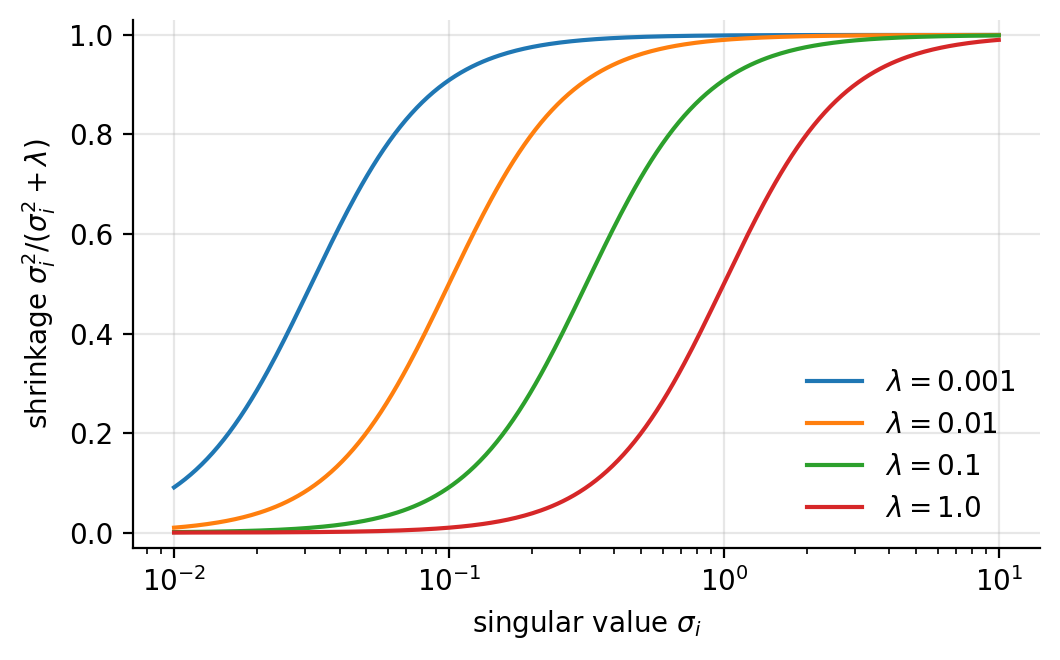
Figure 3.1: The Ridge shrinkage factor \(\sigma_i^{2}/(\sigma_i^{2}+\lambda)\) of Eq. (3.48) against the singular value, for four penalties. The transition is centred on \(\sigma_i=\sqrt{\lambda}\).
An instructive special case. Suppose the design matrix is orthonormal, \(\bm{X}^{T}\bm{X}=\bm{I}\). Then \(\hat{\bm{\theta}}_{\mathrm{OLS}}=\bm{X}^{T}\bm{y}\) and
so every coefficient is scaled by the same factor \(1/(1+\lambda)\) and the estimator tends to zero as \(\lambda\to\infty\). Ridge shrinks all coefficients proportionally; it never sets any of them exactly to zero. Remember this when we reach the Lasso.
Bias and variance. Ridge regression is biased. Taking the expectation of Eq. (3.44) and using \(\mathbb{E}[\bm{y}]=\bm{X}\bm{\theta}\),
for any \(\lambda>0\), the bias growing towards \(-\bm{\theta}\) as \(\lambda\to\infty\). Applying the transformation rule \(\var(\bm{A}\bm{y})=\bm{A}\var(\bm{y})\bm{A}^{T}\) to Eq. (3.44) gives the variance,
which vanishes as \(\lambda\to\infty\). Subtracting the two variances,
and the middle bracket is non-negative definite for \(\lambda>0\), hence so is the whole product. The variance of the Ridge estimator is therefore always smaller than that of OLS.
This is the bias-variance trade-off of Section The bias-variance tradeoff in closed form. Increasing \(\lambda\) increases the squared bias and decreases the variance, monotonically in both cases; by Eq. (2.27) the total error is their sum, and since the variance falls immediately while the bias starts at zero with zero derivative, there always exists a \(\lambda>0\) giving a smaller mean squared error than OLS. Gauss-Markov is not contradicted – the Ridge estimator is not unbiased, so it was never in the competition. Both of the assertions just made can be proved, and the rest of this section does so.
The constrained form, exactly. The correspondence between Eq. (3.43) and the constraint (3.45) is worth stating precisely rather than by assertion, because it is the first appearance of the Karush-Kuhn-Tucker conditions that Chapter 6 will lean on throughout.
Proposition 3.5 (Penalty and constraint)
Let \(t>0\) and let \(\hat{\bm{\theta}}_t\) solve \(\min\|\bm{y}-\bm{X}\bm{\theta}\|_2^{2}\) subject to \(\|\bm{\theta}\|_2^{2}\le t\). If the constraint is active, there is a unique \(\lambda>0\) for which \(\hat{\bm{\theta}}_t\) also solves (3.43), namely the multiplier of the constraint; and conversely, the solution of (3.43) at penalty \(\lambda\) solves the constrained problem with \(t=\|\hat{\bm{\theta}}_{\mathrm{Ridge}}(\lambda)\|_2^{2}\). The map \(\lambda\mapsto\|\hat{\bm{\theta}}_{\mathrm{Ridge}}(\lambda)\|_2^{2}\) is strictly decreasing.
Proof
The Lagrangian of the constrained problem is \(\|\bm{y}-\bm{X}\bm{\theta}\|_2^{2}+\lambda(\|\bm{\theta}\|_2^{2}-t)\), whose stationarity condition in \(\bm{\theta}\) is exactly that of (3.43); the term \(-\lambda t\) does not involve \(\bm{\theta}\) and cannot change the minimiser. Complementary slackness gives \(\lambda>0\) when the constraint is active and \(\lambda=0\) when it is not, and the problem is convex with a strictly feasible point, so the conditions are sufficient as well as necessary. For the monotonicity, Eq. (3.46) gives
in which every term is strictly decreasing in \(\lambda\). \qed
That a useful penalty always exists. Section Ridge regression closed with the assertion that some \(\lambda>0\) gives a smaller mean squared error than ordinary least squares. That statement is due to Hoerl and Kennard and it can be proved in half a page, which is worth doing because the proof shows why the effect is unavoidable rather than fortunate.
Work in the singular basis. Put \(\bm{b}=\bm{V}^{T}\bm{\theta}\) for the true parameter and recall from Eq. (3.46) that the \(i\)th coefficient of the estimator in that basis is \(\sigma_i(\bm{u}_i^{T}\bm{y})/(\sigma_i^{2}+\lambda)\). With \(\bm{y}=\bm{X}\bm{\theta}+\bm{\varepsilon}\) and \(\var(\bm{\varepsilon})=\sigma^{2}\bm{I}\) we have \(\mathbb{E}[\bm{u}_i^{T}\bm{y}]=\sigma_ib_i\) and \(\var(\bm{u}_i^{T}\bm{y})=\sigma^{2}\), so
Because \(\bm{V}\) is orthogonal the total mean squared error of the estimator is the sum over \(i\) of squared bias plus variance,
the first term in the numerator being the squared bias \([\lambda/(\sigma_i^{2}+\lambda)]^{2}b_i^{2}\) and the second the variance.
Theorem 3.6 (Hoerl and Kennard)
Suppose \(\bm{X}\) has full column rank and \(\sigma^{2}>0\). Then \(M'(0)<0\), and consequently there exists \(\lambda>0\) with \(M(\lambda)<M(0)\): some Ridge estimator has a strictly smaller mean squared error than ordinary least squares, whatever the true \(\bm{\theta}\).
Proof
Differentiate Eq. (3.55) term by term. Writing \(N_i(\lambda)=\lambda^{2}b_i^{2}+\sigma^{2}\sigma_i^{2}\) and \(D_i(\lambda)=(\sigma_i^{2}+\lambda)^{2}\),
where the second step cancels the \(\lambda^{2}b_i^{2}\) terms. Setting \(\lambda=0\) leaves \(-2\sigma^{2}\sigma_i^{2}/\sigma_i^{6} =-2\sigma^{2}/\sigma_i^{4}\), so
Since \(M\) is differentiable at \(0\) with a strictly negative derivative, it is strictly smaller than \(M(0)\) for all sufficiently small \(\lambda>0\). \qed
Two things about this proof deserve attention. The bias term contributes nothing to \(M'(0)\): it enters as \(\lambda^{2}\) and so has zero derivative at the origin, while the variance falls linearly. That asymmetry is the whole content of the theorem, and it is Eq. (2.27) speaking again – a little bias is free to second order, and the variance it buys is not. And Eq. (3.56) says the effect is largest exactly when the design is badly conditioned, since the sum is dominated by the smallest singular value. The worse the collinearity, the more Ridge has to offer, which is the practical rule the theorem underwrites. Running the arithmetic on four designs:
     n     p    sigma^2   M(0)=OLS    min_lambda M   best lambda   M'(0) predicted   M'(0) measured
    40     6       1.00      0.1823          0.1636         3.256            -0.0129            -0.0129
    40     6       0.10      0.0214          0.0213        0.1001          -0.001986          -0.001985
    80    20       1.00      0.3461          0.3353         1.363           -0.01642           -0.01642
    25    15       0.50      0.7361          0.6067        0.9295            -0.3386            -0.3386
The minimising penalty is strictly positive in every case, and the numerically measured slope at the origin agrees with Eq. (3.56). The theorem is an existence statement and not a recipe: the optimal \(\lambda\) depends on the unknown \(\bm{b}\) and \(\sigma^{2}\), which is why in practice it is chosen by the cross-validation of Section Cross-validation.
3.9. The Lasso#
Replacing the \(2\)-norm penalty of Eq. (3.43) by a \(1\)-norm gives
which is the Lasso – least absolute shrinkage and selection operator. The change looks slight and its consequences are not: the Lasso sets coefficients exactly to zero, and thereby performs variable selection as part of the fitting, which Ridge regression by Eq. (3.49) never does.
No closed form. Differentiating Eq. (3.57) requires the derivative of the absolute value,
which is undefined at the origin. Ignoring that difficulty for a moment and dropping the \(1/n\), the stationarity condition reads
Because \(\mathrm{sgn}(\bm{\theta})\) depends on the unknown in a non-differentiable way, Eq. (3.59) cannot be solved by a matrix inversion, and no analogue of Eqs. (3.8) or (3.44) exists. The problem is nonetheless convex – a sum of a convex quadratic and a convex norm – so it has a global minimum and can be solved reliably; it is the closed form that is lost, not the solution.
The orthonormal case and soft thresholding. The behaviour becomes transparent in the simplest possible design. Take \(\bm{X}=\bm{I}\) with \(n=p\), so that \(\tilde{\bm{y}}=\bm{\theta}\) and the problem decouples completely into \(p\) scalar problems. For OLS,
For Ridge,
in agreement with Eq. (3.49). For the Lasso,
and treating each \(i\) separately, the derivative for \(\theta_i\neq0\) is \(-2(y_i-\theta_i)+\lambda\,\mathrm{sgn}(\theta_i)=0\). If \(\theta_i>0\) this gives \(\theta_i=y_i-\lambda/2\), which is consistent with \(\theta_i>0\) only when \(y_i>\lambda/2\); if \(\theta_i<0\) it gives \(\theta_i=y_i+\lambda/2\), consistent only when \(y_i<-\lambda/2\). For \(|y_i|\le\lambda/2\) neither branch is consistent and the minimum lies at the kink \(\theta_i=0\). Collecting,
This is the soft thresholding operator, written compactly as
Compare the three results. OLS leaves the coefficient alone. Ridge multiplies it by \(1/(1+\lambda)\), shrinking it towards zero but reaching zero only in the limit \(\lambda\to\infty\). The Lasso subtracts a constant \(\lambda/2\) from its magnitude and truncates at zero, so every coefficient smaller than the threshold is eliminated outright at finite \(\lambda\). The difference between shrinkage and selection is contained in this one comparison.
Why the geometry does it. The constrained forms explain the same fact without any calculus. Ridge minimises the squared error subject to \(\|\bm{\theta}\|_2^{2}\le t\), a ball; the Lasso subject to \(\|\bm{\theta}\|_1\le t\), a cross-polytope – a diamond in two dimensions. The solution lies where the elliptical contours of the squared error first touch the constraint region. A ball has no distinguished points, so the contact occurs at a generic location with all coordinates non-zero. A diamond has corners, and the corners lie on the axes, where some coordinates vanish. Contours are far more likely to meet a protruding corner than a flat face, and every corner is a solution with a zero coefficient. In \(p\) dimensions the \(1\)-norm ball has corners, edges and faces of every dimension, each corresponding to a different set of variables being eliminated.
Figure 3.2 makes the argument concrete for two parameters, where the ball becomes a circle and the diamond a rhombus. Both panels show the same squared-error contours – ellipses centred on the unconstrained minimum \(\hat{\bm{\theta}}_{\mathrm{OLS}}\), with shape set by the Hessian \(\bm{X}^T\bm{X}\) – and the same budget \(t\); the constrained solutions are computed exactly, so the points of contact in the figure are not sketched but solved for. Three things are worth reading off. First, on the circle the touching point is a genuine tangency at a generic location: the Ridge solution is pulled towards the origin, from \((2.0,\,0.5)\) to \((0.92,\,0.39)\) here, but both coordinates survive – shrinkage without selection, exactly as Eq. (3.49) predicted. Second, on the rhombus the first contour to arrive strikes the protruding corner \((t,\,0)\), and the corner lies on an axis: \(\hat\theta_2=0\) exactly, at finite \(t\), with nothing gradual about it. Third – and this is why the Lasso selects so readily – a corner does not need tangency at all. The corner is the solution whenever the negative cost gradient there lies anywhere inside the cone spanned by the normals of its two adjacent edges, so a whole open set of positions of \(\hat{\bm{\theta}}_{\mathrm{OLS}}\) is claimed by each corner, while each point on a smooth boundary claims only the single direction that is exactly normal to it. Selection is the rule, not a lucky accident of where the data happen to lie. The figure also displays the two limits of the constrained problem: shrinking \(t\) towards zero collapses both regions, and both estimators, onto the origin, while any \(t\ge\|\hat{\bm{\theta}}_{\mathrm{OLS}}\|\) (in the corresponding norm) makes the constraint inactive and returns ordinary least squares – the one-to-one correspondence between \(t\) and \(\lambda\) of Proposition 3.5. The normal-cone picture at the corner is precisely the subdifferential condition that the next paragraph derives: Proposition 3.7’s statement that a coefficient stays at zero as long as \(|\tfrac{2}{n}\bm{x}_j^T\bm{r}|\le\lambda\) is the algebraic form of “the gradient points into the cone”.
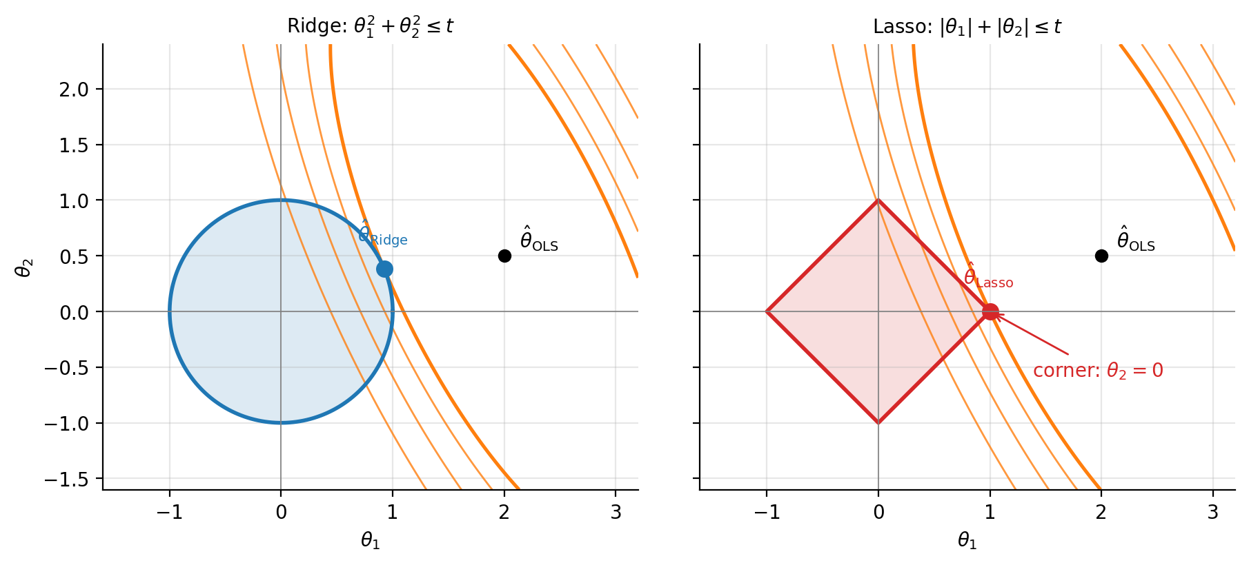
Figure 3.2: The constrained forms of Ridge and Lasso for two parameters. Both panels share the same squared-error contours – ellipses centred on \(\hat{\bm{\theta}}_{\mathrm{OLS}}=(2.0,\,0.5)\) with shape given by the Hessian \(\bm{X}^T\bm{X}\) – and the same budget \(t=1\); the heavier contour is the first to touch each constraint region, and the touching point is the exactly computed constrained solution. On the Ridge circle (left) the contact is a tangency at a generic point and both coordinates remain non-zero. On the Lasso rhombus (right) the contour reaches the corner \((1,\,0)\) first, so that \(\hat\theta_2=0\) exactly: the corner solves the problem for a whole cone of gradient directions, which is the geometric origin of the selection property.
Optimality conditions, done properly. Equation (3.59) was obtained by ignoring the point at which \(\mathrm{sgn}\) is undefined. The difficulty is removed rather than ignored by the subdifferential: for a convex function \(g\), the subdifferential at a point is the set of slopes of all lines lying below the graph and touching it there, and for the absolute value
A convex function is minimised exactly where \(0\) belongs to its subdifferential, which is the generalisation of “the derivative vanishes” and reduces to it wherever the function is differentiable.
Proposition 3.7 (Lasso optimality)
A vector \(\hat{\bm{\theta}}\) minimises the Lasso objective (3.57) if and only if, writing \(\bm{r}=\bm{y}-\bm{X}\hat{\bm{\theta}}\) for the residual and \(\bm{x}_j\) for the \(j\)th column,
Proof
The objective is the sum of the differentiable term \(\|\bm{y}-\bm{X}\bm{\theta}\|_2^{2}/n\), whose gradient is \(-\tfrac{2}{n}\bm{X}^{T}\bm{r}\), and of \(\lambda\|\bm{\theta}\|_1\), whose subdifferential is the product of the sets (3.65) taken coordinatewise. For a sum of a differentiable convex function and a convex one the subdifferential is the sum of the two, so \(\bm{0}\) lies in it exactly when \(\tfrac{2}{n}\bm{x}_j^{T}\bm{r}\in\lambda\,\partial|\hat{\theta}_j|\) for every \(j\), which is Eq. (3.66). \qed
Read the second half of Eq. (3.66) again, because it is the selection property in its exact form. A coefficient is zero not by accident but because its column’s correlation with the residual is too small to pay the price \(\lambda\); the variable is excluded as long as it fails to earn its penalty. Two corollaries follow immediately.
Proposition 3.8 (The penalty that kills everything)
The solution is \(\hat{\bm{\theta}}=\bm{0}\) if and only if
Proof
Put \(\hat{\bm{\theta}}=\bm{0}\) in Eq. (3.66). The residual is then \(\bm{y}\), every coefficient is zero, and the second condition reads \(|\tfrac{2}{n}\bm{x}_j^{T}\bm{y}|\le\lambda\) for all \(j\), which is Eq. (3.67). Since the conditions are necessary and sufficient, the equivalence is exact. \qed
Equation (3.67) is why every Lasso implementation computes a path of solutions on a geometric grid running down from \(\lambda_{\max}\): above it there is nothing to compute, and below it the solution changes continuously.
Proposition 3.9 (The fit is unique even when the coefficients are not)
If \(\hat{\bm{\theta}}^{(1)}\) and \(\hat{\bm{\theta}}^{(2)}\) both minimise Eq. (3.57), then \(\bm{X}\hat{\bm{\theta}}^{(1)}=\bm{X}\hat{\bm{\theta}}^{(2)}\) and \(\|\hat{\bm{\theta}}^{(1)}\|_1=\|\hat{\bm{\theta}}^{(2)}\|_1\).
Proof
Let \(c^{\star}\) be the common minimum value and consider the midpoint \(\bar{\bm{\theta}}=\tfrac12(\hat{\bm{\theta}}^{(1)}+\hat{\bm{\theta}}^{(2)})\). The \(1\)-norm is convex, so \(\|\bar{\bm{\theta}}\|_1\le\tfrac12\|\hat{\bm{\theta}}^{(1)}\|_1 +\tfrac12\|\hat{\bm{\theta}}^{(2)}\|_1\). The squared error is strictly convex along any direction in which \(\bm{X}\bm{\theta}\) changes, so if \(\bm{X}\hat{\bm{\theta}}^{(1)}\neq\bm{X}\hat{\bm{\theta}}^{(2)}\) then the squared error at the midpoint is strictly less than the average of the two. Adding the two inequalities gives an objective value at \(\bar{\bm{\theta}}\) strictly below \(c^{\star}\), a contradiction. Hence the fits coincide, the squared-error terms are equal, and the \(1\)-norms must therefore be equal too. \qed
This is the precise sense in which the instability noted in the notebox below is a property of the parameterisation and not of the prediction. With two identical columns the Lasso may place all the weight on either, or split it, and every such choice has the same \(1\)-norm and gives the same fitted values; what is arbitrary is the attribution, not the answer.
Coordinate descent. Equation (3.63) is exact only for an orthonormal design, but it suggests the algorithm that solves the general problem. Suppose we fix all coefficients but one and minimise over \(\theta_j\) alone. Writing the partial residual with the \(j\)th contribution removed,
where \(\bm{x}_k\) is column \(k\), the one-dimensional problem is exactly of the form solved above, and its answer is
which for standardised columns has \(\bm{x}_j^{T}\bm{x}_j=n\). Cycling through
the coordinates until the parameters stop changing is coordinate
descent, and because the cost is convex and the non-differentiable part is
separable – it is a sum of terms each involving one coordinate – the
procedure is guaranteed to converge to the global minimum. This is what
sklearn.linear_model.Lasso runs. The reader will recognise the
pattern from the Gauss-Seidel iteration of Eq. (1.92):
update one coordinate at a time, using the most recent values of all the
others.
import numpy as np

def soft_threshold(z, gamma):
    """Soft thresholding operator S_gamma(z), Eq. (3.softthresholdop)."""
    return np.sign(z) * np.maximum(np.abs(z) - gamma, 0.0)


def lasso_coordinate_descent(X, y, lmbda, n_iter=1000, tol=1e-8):
    """Lasso by cyclic coordinate descent.

    Minimises ||y - X theta||^2 / n + lmbda * ||theta||_1.
    The columns of X are assumed centred and standardised, and no
    intercept is penalised -- see Section on scaling and the intercept.
    """
    n, p = X.shape
    theta = np.zeros(p)
    col_norms = np.sum(X**2, axis=0)
    r = y - X @ theta                              # full residual

    for _ in range(n_iter):
        theta_old = theta.copy()
        for j in range(p):
            # partial residual: add back the current contribution of column j
            r += X[:, j] * theta[j]
            rho = X[:, j] @ r
            theta[j] = soft_threshold(rho, lmbda * n / 2.0) / col_norms[j]
            r -= X[:, j] * theta[j]                # remove the updated one
        if np.max(np.abs(theta - theta_old)) < tol:
            break

    return theta
Machine learning connection
The selection property makes the Lasso the natural first tool when \(p\) is large and most features are believed irrelevant – gene expression studies, text features, high-order polynomial bases. It has real limitations. When several features are strongly correlated the Lasso tends to pick one arbitrarily and discard the rest, which is unstable under resampling and misleading if the discarded features are scientifically meaningful; when \(p>n\) it can select at most \(n\) variables. The elastic net, which penalises \(\alpha\|\bm{\theta}\|_1+(1-\alpha)\|\bm{\theta}\|_2^{2}\), was designed to repair both defects by combining selection with the grouping behaviour of Ridge. Note finally that the sparsity is a property of the \(1\)-norm, not of regression: the same penalty produces sparse solutions in compressed sensing, in dictionary learning and in the pruning of neural networks.
3.10. Comparing the three estimators#
It is worth seeing the three methods act on the same small problem. Take the targets and design matrix
so that there are three observations, two features and two parameters. The third row contributes nothing to the fit but does contribute to the error, which is what makes the example non-trivial. Since \(\bm{X}\bm{\theta}=(2\theta_0,\theta_1,0)^{T}\), the unpenalised cost is
minimised at
Adding the Ridge penalty gives \(C(\bm{\theta})=(4-2\theta_0)^{2}+(2-\theta_1)^{2} +\lambda(\theta_0^{2}+\theta_1^{2})\) up to the constant, and differentiating with respect to each parameter separately,
which reproduces Eq. (3.72) at \(\lambda=0\) and decays to zero as \(\lambda\) grows. Notice that the two coefficients are shrunk by different factors, \(4/(4+\lambda)\) and \(1/(1+\lambda)\): the penalty is applied uniformly in parameter space, but the curvature of the cost differs between directions, so the coefficient belonging to the better-determined feature resists shrinkage more strongly. This is Eq. (3.48) with \(\sigma_0^2=4\) and \(\sigma_1^2=1\). Neither coefficient ever becomes exactly zero.
The Lasso behaves differently. Because the problem is diagonal, each coefficient can be treated separately as in Eq. (3.63): differentiating \((2-\theta_1)^{2}+\lambda|\theta_1|\) gives \(\theta_1=\max(2-\lambda/2,\,0)\), while \((4-2\theta_0)^{2}+\lambda|\theta_0|\) gives \(\theta_0=\max\left((16-\lambda)/8,\,0\right)\). The first coefficient is eliminated at \(\lambda=4\) and the second at \(\lambda=16\), both at finite \(\lambda\) and both exactly. Plotting all three coefficient paths against \(\lambda\) shows the distinction at a glance: the Ridge curves approach the axis asymptotically, the Lasso curves reach it and stop.
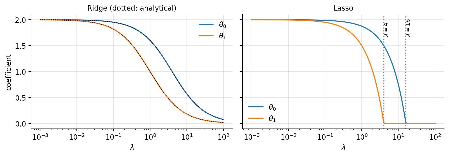
Figure 3.3: Coefficient paths for the toy problem (3.70). The Ridge coefficients (left) follow the analytical result (3.73), shown dotted, and approach zero only asymptotically. The Lasso coefficients (right) reach zero at the finite thresholds \(\lambda=4\) and \(\lambda=16\) predicted by Eq. (3.63).
import numpy as np
import matplotlib.pyplot as plt
from sklearn.linear_model import Ridge, Lasso

X = np.array([[2.0, 0.0], [0.0, 1.0], [0.0, 0.0]])
y = np.array([4.0, 2.0, 3.0])

n = X.shape[0]
lambdas = np.logspace(-3, 2, 200)

# scikit-learn's Ridge minimises ||y - X t||^2 + alpha ||t||^2, so alpha = lambda,
# but its Lasso minimises ||y - X t||^2 / (2n) + alpha ||t||_1, so alpha = lambda / (2n).
ridge_path = np.array([Ridge(alpha=l, fit_intercept=False).fit(X, y).coef_
                       for l in lambdas])
lasso_path = np.array([Lasso(alpha=l / (2 * n), fit_intercept=False,
                             max_iter=100000).fit(X, y).coef_
                       for l in lambdas])

# Analytical results: Eq. (3.toyridge) for Ridge, Eq. (3.softthreshold) for Lasso
ridge_exact = np.column_stack([8.0 / (4.0 + lambdas), 2.0 / (1.0 + lambdas)])
lasso_exact = np.column_stack([np.maximum((16.0 - lambdas) / 8.0, 0.0),
                               np.maximum(2.0 - lambdas / 2.0, 0.0)])
assert np.allclose(ridge_path, ridge_exact) and np.allclose(lasso_path, lasso_exact)

fig, ax = plt.subplots(1, 2, figsize=(10, 4), sharey=True)
for k in range(2):
    ax[0].semilogx(lambdas, ridge_path[:, k], label=rf"$\theta_{k}$")
    ax[1].semilogx(lambdas, lasso_path[:, k], label=rf"$\theta_{k}$")
ax[0].set_title("Ridge"); ax[1].set_title("Lasso")
for a in ax:
    a.set_xlabel(r"$\lambda$"); a.legend()
plt.show()
The two rescalings in that code deserve attention, because they are exactly
the trap warned against in Section Scaling, centring and the intercept.
scikit-learn minimises
\(\|\bm{y}-\bm{X}\bm{\theta}\|_2^{2}+\alpha\|\bm{\theta}\|_2^{2}\) for Ridge but
\(\|\bm{y}-\bm{X}\bm{\theta}\|_2^{2}/(2n)+\alpha\|\bm{\theta}\|_1\) for the
Lasso – the same library uses different conventions for the two
methods, so \(\alpha=\lambda\) in one case and \(\alpha=\lambda/(2n)\) in the
other. With the conversions in place the computed paths agree with the
analytical results (3.73) and (3.63) to
machine precision, which is what the assertion checks. Such factors differ
between every implementation and every textbook, and reconciling one’s own
code with a library means checking them explicitly rather than assuming.
3.11. A Bayesian reading#
The three estimators can be derived a second time, from a viewpoint in which the parameters rather than the data are random. The unification is elegant, and it explains where the penalties come from rather than merely postulating them.
Bayes’ theorem. From the product rule for joint probabilities, \(p(X,Y)=p(X\mid Y)p(Y)=p(Y\mid X)p(X)\), we obtain immediately
dropping the normalisation \(p(\bm{D})\), which does not depend on \(\bm{\theta}\). The left-hand side is the posterior, the probability of the parameters given the data; on the right are the likelihood \(p(\bm{D}\mid\bm{\theta})\), which we already modelled in Eq. (3.25), and the prior \(p(\bm{\theta})\), which encodes what we believed about the parameters before seeing any data. Choosing the \(\bm{\theta}\) that maximises the posterior is maximum-a-posteriori (MAP) estimation.
A Gaussian prior gives Ridge. Suppose we believe, before seeing the data, that the parameters are small: independent, zero-mean Gaussians of variance \(\tau^{2}\),
The posterior is then the product of Eq. (3.25) and Eq. (3.75). Taking the negative logarithm and discarding terms independent of \(\bm{\theta}\),
which, on identifying \(\lambda=\sigma^{2}/\tau^{2}\) after multiplying through by \(2\sigma^2\), is exactly the Ridge cost function (3.43).
A Laplace prior gives the Lasso. Replace the Gaussian prior by a Laplace (double exponential) distribution with zero mean,
The same steps give
the Lasso cost function (3.57). A flat prior, expressing no preference at all, leaves only the likelihood and returns ordinary least squares.
What the unification tells us. The strength of the prior and the strength of the penalty are the same quantity. A large \(\lambda\) corresponds to a small prior variance – a firm belief that the coefficients are near zero – and a small \(\lambda\) to a diffuse prior that lets the data speak. The difference between Ridge and the Lasso is now visibly a difference between two prior shapes: the Laplace density has a sharp peak at the origin and heavier tails than the Gaussian, so it simultaneously expresses a stronger belief that coefficients are exactly zero and a greater tolerance for the few that are large. That is precisely the behaviour of Eq. (3.63).
It should be said that MAP estimation is not the whole of Bayesian inference. It returns a single point, the mode of the posterior, and discards the distribution around it – which is the part a Bayesian would consider the answer. A full treatment would report the posterior itself, giving credible intervals directly rather than through the sampling argument of Eq. (3.34), and would integrate over \(\bm{\theta}\) when making predictions instead of fixing it at the mode. We return to this when we discuss Bayesian neural networks and the Gaussian processes for which the Cholesky factorisation of Section LU and Cholesky decompositions was introduced.
3.12. Kernel methods: regression without coordinates#
Every model in this chapter is linear in the parameters and can be made non-linear in the inputs by the basis expansion of Section The linear model and the design matrix: replace \(\bm{x}\) by \(\bm{\phi}(\bm{x})\) and fit a linear model in the enlarged space. The difficulty is arithmetic. A quadratic expansion of \(d\) inputs has \(\bigO(d^{2})\) features, a cubic one \(\bigO(d^{3})\), and the map one would often like to use has infinitely many. This section shows that for Ridge regression the expansion need never be carried out, that the resulting method is an exact rewriting and not an approximation, and that the same device is the one Chapter 6 uses for support vector machines and Section Kernel logistic regression for logistic regression. It also shows, because it is true and usually left unsaid, that the device does not work for the Lasso.
3.12.1. An identity that moves the problem#
Everything rests on one line of algebra.
Lemma 3.10 (The push-through identity)
For any \(\bm{X}\in\mathbb{R}^{n\times p}\) and any \(\lambda>0\),
Both inverses exist, the left of a \(p\times p\) matrix and the right of an \(n\times n\) one.
Proof
Both matrices being inverted are symmetric with eigenvalues at least \(\lambda\), hence invertible. Start from the trivial identity
in which the middle expression is read in two ways. Multiplying on the left by \((\bm{X}^{T}\bm{X}+\lambda\bm{I}_p)^{-1}\) and on the right by \((\bm{X}\bm{X}^{T}+\lambda\bm{I}_n)^{-1}\) gives Eq. (3.79). \qed
The name is descriptive: \(\bm{X}^{T}\) is pushed through the inverse, and in doing so the matrix that must be inverted changes size from \(p\) to \(n\). The identity fails for \(\lambda=0\), which is the first hint that a penalty is not optional here.
Theorem 3.11 (The dual form of Ridge regression)
The Ridge estimator (3.44) satisfies
so that the fitted function at a new point is
Proof
Apply Lemma 3.10 to Eq. (3.44): \(\hat{\bm{\theta}}=(\bm{X}^{T}\bm{X}+\lambda\bm{I})^{-1}\bm{X}^{T}\bm{y} =\bm{X}^{T}(\bm{X}\bm{X}^{T}+\lambda\bm{I})^{-1}\bm{y}=\bm{X}^{T}\bm{\alpha}\). Equation (3.82) is then \(\bm{x}^{T}\bm{X}^{T}\bm{\alpha}\) written out. \qed
Look at what Eqs. (3.81) and (3.82) contain. The matrix \(\bm{K}\) has entries \(K_{ij}=\bm{x}_i^{T}\bm{x}_j\); the prediction needs \(\bm{x}_i^{T}\bm{x}\). The data enter only through inner products. The individual vectors \(\bm{x}_i\) are never needed once the \(n\times n\) matrix of their inner products is known, and the parameter vector \(\hat{\bm{\theta}}\) – which lives in the feature space and may be enormous – is never formed. The estimator has been rewritten in terms of \(n\) numbers \(\alpha_i\), one per observation, instead of \(p\) numbers \(\theta_j\), one per feature.
=== 1. the push-through identity, Lemma 3.pushthrough ===
     n     p   lambda   max |LHS - RHS|   ||theta_p - theta_n||
    20     5     0.01         4.012e-14               8.120e-14
    20    50     0.01         1.386e-13               4.110e-13
   200     3     0.01         1.817e-13               3.997e-13
    50    50     0.01         1.989e-13               2.683e-12
3.12.2. Kernels#
Now perform the basis expansion. Fitting Ridge regression to the expanded design matrix \(\bm{\Phi}\) with rows \(\bm{\phi}(\bm{x}_i)^{T}\), Theorem 3.11 gives the same formulas with \(K_{ij}=\bm{\phi}(\bm{x}_i)^{T}\bm{\phi}(\bm{x}_j)\). Define the kernel
which is the same object as Eq. (6.30) in the chapter on support vector machines. Then
is kernel ridge regression. Its cost is the \(\bigO(n^{3})\) of one linear solve, whatever the dimension of \(\bm{\phi}\) – including infinite.
The reason this is not a swindle is that for many useful maps the inner product has a closed form which is cheaper than the map. For the quadratic map of Eq. (6.28) the kernel is \((\bm{x}^{T}\bm{x}')^{2}\); the polynomial and Gaussian kernels of Section Common kernels and Mercer’s theorem are the standard choices, and Mercer’s theorem stated there says exactly which functions \(k\) arise from some \(\bm{\phi}\) in this way: the symmetric positive semi-definite ones. Everything in Section Common kernels and Mercer’s theorem applies verbatim here, and nothing in this section is specific to regression.
=== 3. kernel ridge regression, Theorem 3.krr ===
  (a) the quadratic kernel against its explicit feature map
      max |k(x,x') - phi(x).phi(x')| : 1.421e-14
      max |f_kernel(x) - f_primal(x)|: 1.915e-14
The second line is the claim of this section, measured: the function obtained
from the \(6\times6\) primal system with an explicit feature map and the function
obtained from the \(60\times60\) kernel system are the same function. Against
scikit-learn, whose \verb!KernelRidge! solves the identical system
with its \verb!alpha! playing the part of our \(\lambda\):
  (b) the Gaussian kernel, ours against scikit-learn
      gamma   lambda    our test MSE   sklearn test MSE   max |f_ours - f_sk|
       0.25    0.001       0.008634           0.008634            1.847e-13
       1.00    0.001       0.056491           0.056491            8.349e-14
       4.00    0.100       0.037478           0.037478            1.277e-15
import numpy as np

def gaussian_kernel(A, B, gamma):
    """k(x,x') = exp(-gamma ||x - x'||^2), the Gaussian kernel of Section 6.mercer."""
    d2 = (A**2).sum(1)[:, None] + (B**2).sum(1)[None, :] - 2.0 * A @ B.T
    return np.exp(-gamma * np.maximum(d2, 0.0))


def kernel_ridge_fit(K, y, lmbda):
    """alpha = (K + lambda I)^{-1} y, Eq. (3.krr).  One n x n solve."""
    return np.linalg.solve(K + lmbda * np.eye(len(y)), y)


def kernel_ridge_predict(alpha, Xtrain, Xnew, gamma):
    """f(x) = sum_i alpha_i k(x_i, x), Eq. (3.krr)."""
    return gaussian_kernel(Xnew, Xtrain, gamma) @ alpha
Which side to solve
Theorem 3.11 gives two routes to the same estimator, and the choice between them is arithmetic. The primal system is \(p\times p\) and the dual \(n\times n\), so the primal wins whenever \(p<n\) and the dual whenever \(p>n\); with a thousand observations and ten features one should never form a kernel matrix, and with a hundred observations and a million features one should never form \(\bm{X}^{T}\bm{X}\). The kernel route additionally costs \(\bigO(n^{2})\) memory, which is what limits it to sample sizes in the tens of thousands and is the reason for the approximations of Section There is no kernel Lasso. A method that scales with the number of observations rather than the number of features is not automatically an improvement; it is a different trade.
3.12.3. Why the same trick works for any loss: the representer theorem#
Theorem 3.11 was proved by an algebraic identity special to the squared error. The result is far more general, and stating it in the general form is what allows Chapters 5 and 6 to use it without repeating the derivation.
Let \(\mathcal{H}\) be the space of functions spanned by \(\{k(\bm{x},\cdot)\}\) with the inner product determined by \(\langle k(\bm{x},\cdot),k(\bm{x}',\cdot)\rangle=k(\bm{x},\bm{x}')\) – the reproducing kernel Hilbert space of \(k\). The name records its one essential property, that \(\langle f,k(\bm{x},\cdot)\rangle=f(\bm{x})\) for every \(f\in\mathcal{H}\): evaluation at a point is an inner product.
Theorem 3.12 (Representer theorem)
Let \(L\) be any function of its arguments and let \(\Omega\) be strictly increasing on \([0,\infty)\). Then every minimiser of
admits the finite expansion
for some \(\bm{\alpha}\in\mathbb{R}^{n}\).
Proof
Let \(\mathcal{S}\) be the span of \(k(\bm{x}_0,\cdot),\dots,k(\bm{x}_{n-1},\cdot)\) and decompose any \(f\in\mathcal{H}\) orthogonally as \(f=f_{\parallel}+f_{\perp}\) with \(f_{\parallel}\in\mathcal{S}\) and \(f_{\perp}\perp\mathcal{S}\). By the reproducing property,
so the component \(f_{\perp}\) has no effect whatever on the data-fitting term: the loss sees only \(f_{\parallel}\). It does affect the penalty, since by orthogonality \(\|f\|^{2}_{\mathcal{H}}=\|f_{\parallel}\|^{2}_{\mathcal{H}} +\|f_{\perp}\|^{2}_{\mathcal{H}}\ge\|f_{\parallel}\|^{2}_{\mathcal{H}}\), with equality only when \(f_{\perp}=0\). Since \(\Omega\) is strictly increasing, deleting \(f_{\perp}\) leaves the loss unchanged and strictly decreases the penalty unless it was already zero. A minimiser therefore has \(f_{\perp}=0\), that is \(f\in\mathcal{S}\), which is Eq. (3.86). \qed
This is a remarkable statement and it is worth pausing on. The minimisation is over an infinite-dimensional space of functions; the answer is guaranteed to lie in the \(n\)-dimensional subspace spanned by the kernel evaluated at the training points. The data determine the dimension of the problem, not the model. With the squared loss and \(\Omega(t)=\tfrac{\lambda}{2}t^{2}\) the theorem reproduces Eq. (3.84); with the logistic loss it gives the kernel logistic regression of Section Kernel logistic regression; with the hinge loss it gives the support vector machine of Chapter 6, whose expansion (6.33) over support vectors is Eq. (3.86) with most coefficients equal to zero. Why the hinge loss and only the hinge loss produces those zeros is Theorem 6.1.
3.12.4. There is no kernel Lasso#
It is natural to ask for the same treatment of the Lasso, and the request appears in the literature under the name kernel Lasso. The honest answer is that the construction that works for Ridge regression does not exist here, and it is worth being precise about why, because the reason is instructive rather than technical.
Theorem 3.12 requires the penalty to be a strictly increasing function of \(\|f\|_{\mathcal{H}}\). The Lasso penalty is \(\|\bm{\theta}\|_1\), a function not of \(f\) but of the coordinates of \(f\) in the feature space – and those coordinates are not determined by the kernel.
Proposition 3.13 (The \(1\)-norm is not a property of the function)
Let \(\bm{\phi}\) be a feature map for \(k\) and let \(\bm{R}\) be any orthogonal matrix on the feature space. Then \(\bm{R}\bm{\phi}\) is also a feature map for \(k\), the two parameterisations \(\bm{\theta}\) and \(\bm{R}\bm{\theta}\) describe the same function, and
Consequently \(\|\bm{\theta}\|_1\) is not a functional of \(f\), and no penalty built from it can be expressed through the kernel alone.
Proof
Two lines of algebra:
so \(\bm{R}\bm{\phi}\) has the same kernel and describes the same function. The \(2\)-norm is invariant because \(\bm{R}\) is orthogonal. The \(1\)-norm is not invariant under rotations – a rotation by \(\pi/4\) turns \((1,0)\), of \(1\)-norm one, into \((\tfrac{1}{\sqrt2},\tfrac{1}{\sqrt2})\), of \(1\)-norm \(\sqrt2\). \qed
Measured on the quadratic feature map of this chapter’s example, with a random orthogonal \(\bm{R}\):
     quantity                                value (phi)    value (R phi)
     ||theta||_2                              0.302326         0.302326
     ||theta||_1                              0.414053         0.637376
     max |f(x) - f_rotated(x)| on test       5.551e-16
The two weight vectors describe the same function to machine precision and disagree in \(1\)-norm by more than fifty per cent. A Lasso in feature space is therefore not a well-posed problem given only a kernel: it depends on which square root of \(\bm{K}\) one happens to have chosen, and Mercer’s theorem supplies no canonical choice. Two repairs are available, and they do different things.
Repair one: penalise the dual coefficients. Take the representation (3.86) as given and put the \(1\)-norm on \(\bm{\alpha}\) instead of on \(\bm{\theta}\):
This is well posed – \(\bm{\alpha}\) is determined by the kernel – and it is nothing more mysterious than an ordinary Lasso whose design matrix happens to be the Gram matrix. Everything proved in Section The Lasso therefore applies unchanged: Proposition 3.7 gives the optimality conditions with \(\bm{x}_j\) replaced by the \(j\)th column \(\bm{k}_j\) of \(\bm{K}\),
Proposition 3.8 gives \(\mu_{\max}=\tfrac{2}{n}\|\bm{K}^{T}\bm{y}\|_\infty\), and the coordinate descent of Eq. (3.69) solves it.
What must be understood is what is being selected. The columns of \(\bm{K}\) are indexed by training points, so Eq. (3.88) is sparse in the examples and not in the features: it discards data points, not variables. That is a useful thing – it produces a prediction rule that evaluates the kernel at a handful of points rather than all \(n\), which is exactly the economy support vectors provide in Chapter 6 – but it is not what the Lasso does in Section The Lasso, and calling both by the same name has caused a good deal of confusion.
      mu      non-zero alpha of 60   train MSE   max KKT violation
    0.0001                     28    0.002055           1.266e-06
    0.0010                     20    0.003362           1.416e-07
    0.0100                      7    0.008227           2.227e-13
    0.1000                      3    0.059848           1.688e-13
def kernel_lasso(K, y, mu, n_iter=20000, tol=1e-12):
    """Cyclic coordinate descent on ||y - K a||^2 / n + mu ||a||_1.

    Identical to lasso_coordinate_descent above with the Gram matrix as the
    design; the solution is sparse in the training points, Eq. (3.klasso).
    """
    n = len(y)
    a = np.zeros(n)
    cn = (K**2).sum(0)
    r = y - K @ a
    for _ in range(n_iter):
        a_old = a.copy()
        for j in range(n):
            r += K[:, j] * a[j]
            a[j] = soft_threshold(K[:, j] @ r, mu * n / 2.0) / cn[j]
            r -= K[:, j] * a[j]
        if np.abs(a - a_old).max() < tol:
            break
    return a
The last column above is the largest violation of Eq. (3.89) at the returned solution, and it is the check that should accompany any implementation of a non-differentiable problem: an optimality condition that can be evaluated is worth more than a convergence message. The measured \(\mu_{\max}\) for this problem is \(0.290436\), and the solver returns exactly zero non-zero coefficients just above it, as Proposition 3.8 requires.
Repair two: build the feature map explicitly, then use the Lasso. If sparsity in features is what is wanted, the honest route is to construct an explicit finite map \(\bm{z}(\bm{x})\in\mathbb{R}^{m}\) whose inner products approximate the kernel, \(\bm{z}(\bm{x})^{T}\bm{z}(\bm{x}')\approx k(\bm{x},\bm{x}')\), and then run the ordinary Lasso of Section The Lasso in that basis. Two constructions are standard. The Nystr”om map picks \(m\) landmark points, forms the \(m\times m\) kernel matrix \(\bm{K}_{mm}\) among them, and sets \(\bm{Z}=\bm{K}_{nm}\bm{K}_{mm}^{-1/2}\); it is exact when the landmarks are all \(n\) points. Random Fourier features exploit Bochner’s theorem, which represents a shift-invariant kernel as the Fourier transform of a probability measure, and estimate that integral by sampling \(m\) frequencies.
Both make an approximation the exact kernel method does not make, and both give back what the exact method cannot: a finite, named set of features among which the \(1\)-norm can genuinely select. A Nystr”om feature is a landmark point and a Fourier feature is a frequency, so the selected set is interpretable in a way that a sparse \(\bm{\alpha}\) is not.
      method             m    max |Z Z^T - K|   Lasso non-zeros   test MSE
      Nystrom          10         9.937e-01                 9    0.026111
      Nystrom          30         2.947e-01                18    0.013798
      Nystrom          60         6.439e-15                22    0.012815
      Fourier          64         4.371e-01                18    0.013377
      Fourier         256         1.668e-01                14    0.001599
      Fourier        1024         1.105e-01                11    0.000907
The Nystr”om map reproduces the Gram matrix exactly once \(m=n\), as it must; the random map converges only in expectation and slowly, its error falling like \(m^{-1/2}\), which is the price of not looking at the data when choosing the features.
Machine learning connection
The pattern of this section recurs throughout the book and is worth naming. A method is characterised by a penalty, and a penalty is meaningful only relative to a parameterisation. The \(2\)-norm survives a change of orthonormal basis and can therefore be expressed through the kernel, which is why Ridge regression kernelises and why the RKHS norm is the natural penalty on functions. The \(1\)-norm does not survive, which is why the Lasso is a statement about a chosen set of features and cannot be lifted to a statement about a function. When a regulariser is proposed, the first question to ask is what it is invariant under, because that determines what it can be a penalty on.
3.13. Scaling, centring and the intercept#
We now address a set of practical questions which cause more confusion than any of the mathematics above, and which are the usual reason a hand-written implementation disagrees with a library.
Why scaling matters for penalised regression. The penalties \(\|\bm{\theta}\|_2^{2}\) and \(\|\bm{\theta}\|_1\) treat all coefficients alike, but a coefficient’s magnitude depends on the units of its feature. Suppose one predictor is a person’s height. Measured in millimetres the fitted coefficient is a thousand times smaller than the same coefficient measured in metres, and it is therefore penalised a thousand times less. The consequence is stark: for Ridge and the Lasso, a change of units is not a harmless relabelling but a change of model. Unless the features are already on comparable scales, they must be standardised – each column centred and divided by its standard deviation, as in Section Arrays in practice: numpy, BLAS and LAPACK – before a penalty is applied. Ordinary least squares is exempt, since Eq. (3.8) is equivariant under rescaling of the columns; the fitted values do not change, only the coefficients, in a compensating way.
Why OLS is equivariant – and why the penalised methods are not. Both claims of the previous paragraph deserve proof, and the proofs are three lines each. A change of units multiplies each column of the design matrix by a positive constant: measuring feature \(j\) in units a factor \(d_j\) smaller turns the column \(\bm{x}_j\) into \(d_j\bm{x}_j\) (a length recorded in millimetres rather than metres has \(d_j=1000\)). Collecting the factors in \(\bm{D}=\mathrm{diag}(d_0,\dots,d_{p-1})\), the design matrix becomes \(\bm{X}\bm{D}\), and a new input rescales the same way. For ordinary least squares, assuming full column rank,
using that diagonal matrices commute with themselves and invert entrywise. The coefficients rescale by exactly the inverse factors – a slope per millimetre is a thousandth of a slope per metre – and every prediction is untouched: the fitted values are \(\bm{X}\bm{D}\,\bm{D}^{-1}\hat{\bm{\theta}}=\bm{X}\hat{\bm{\theta}}\), and a new point \(\bm{x}_*\), which in the new units reads \(\bm{D}\bm{x}_*\), predicts \((\bm{D}\bm{x}_*)^T\bm{D}^{-1}\hat{\bm{\theta}}=\bm{x}_*^T\hat{\bm{\theta}}\). This is equivariance: the parametrisation moves, the model does not.
For Ridge regression the same computation tells a different story. Factor the regularised matrix as \(\bm{D}\bm{X}^T\bm{X}\bm{D}+\lambda\bm{I} = \bm{D}\left(\bm{X}^T\bm{X}+\lambda\bm{D}^{-2}\right)\bm{D}\); inverting and multiplying by \(\bm{D}\bm{X}^T\bm{y}\) gives
The rescaled problem is therefore not the original Ridge problem in disguise: it is ordinary-units Ridge with the spherical penalty \(\lambda\|\bm{\theta}\|_2^2\) replaced by the axis-weighted penalty \(\lambda\,\bm{\theta}^T\bm{D}^{-2}\bm{\theta}\) – an ellipsoid whose axes are set by the units. The fitted values \(\bm{X}(\bm{X}^T\bm{X}+\lambda\bm{D}^{-2})^{-1}\bm{X}^T\bm{y}\) change unless \(\bm{D}\) is a multiple of the identity (a uniform rescaling only relabels \(\lambda\) as \(\lambda/d^2\) and stays within the Ridge family; it is the relative scales of the features that change the model). For the Lasso the substitution \(\bm{\theta}=\bm{D}\bm{\theta}'\) in the rescaled objective gives
each feature now pays its own price \(\lambda/d_j\), and the feature recorded in millimetres pays a thousandth of what it paid in metres. A change of units is a change of the penalty, hence of the model – which coefficients are shrunk, and which are selected, becomes an artefact of the bookkeeping. The following program shows all three statements at work on one small data set, with the intercept handled by centring as derived below.
import numpy as np
from sklearn.linear_model import Lasso

rng = np.random.default_rng(2026)
n = 50
x1 = rng.random(n)                     # a length, measured in metres
x2 = rng.random(n)                     # a time, measured in seconds
y = 2.0 * x1 - 3.0 * x2 + 0.1 * rng.standard_normal(n)

X = np.column_stack([x1, x2])
D = np.diag([1000.0, 1.0])             # metres -> millimetres in column 1
XD = X @ D                             # the same data, in the new units

Xc, yc = X - X.mean(axis=0), y - y.mean()      # centred: intercept handled
XDc = XD - XD.mean(axis=0)                     # separately and unpenalised

lmbda = 0.1
def ols(X, y):
    return np.linalg.lstsq(X, y, rcond=None)[0]
def ridge(X, y, P):                    # generalised penalty lambda theta^T P theta
    return np.linalg.solve(X.T @ X + lmbda * P, X.T @ y)

I = np.eye(2)
t, tD = ols(Xc, yc), ols(XDc, yc)
print("OLS   coefficients (m,s):", t, "  (mm,s):", tD)
print("OLS   D theta_mm = theta_m:", np.allclose(np.diag(D) * tD, t),
      "  max |prediction change|: %.2e" % np.max(np.abs(XDc @ tD - Xc @ t)))

r, rD = ridge(Xc, yc, I), ridge(XDc, yc, I)
print("Ridge coefficients (m,s):", r, "  (mm,s):", rD)
print("Ridge max |prediction change|: %.3f" % np.max(np.abs(XDc @ rD - Xc @ r)))
r_mod = ridge(Xc, yc, np.linalg.inv(D @ D))    # penalty lambda theta^T D^-2 theta
print("Ridge on XD = modified-penalty ridge on X:",
      np.allclose(np.diag(D) * rD, r_mod))

la = Lasso(alpha=lmbda / 2, fit_intercept=False, max_iter=100000)
lm, lmm = la.fit(Xc, yc).coef_.copy(), la.fit(XDc, yc).coef_.copy()
print("Lasso coefficients (m,s):", lm, "  (mm,s):", lmm)
print("Lasso max |prediction change|: %.3f" % np.max(np.abs(XDc @ lmm - Xc @ lm)))
OLS   coefficients (m,s): [ 1.98213925 -2.97802972]   (mm,s): [ 1.98213925e-03 -2.97802972e+00]
OLS   D theta_mm = theta_m: True   max |prediction change|: 8.88e-16
Ridge coefficients (m,s): [ 1.91639278 -2.90255695]   (mm,s): [ 1.98248632e-03 -2.90233356e+00]
Ridge max |prediction change|: 0.033
Ridge on XD = modified-penalty ridge on X: True
Lasso coefficients (m,s): [ 1.12291528 -2.32899154]   (mm,s): [ 1.98426741e-03 -2.32600432e+00]
Lasso max |prediction change|: 0.426
The output is the two propositions in numerical form. For OLS the millimetre coefficient is exactly a thousandth of the metre coefficient and the predictions agree to machine precision. For Ridge the predictions move – and the third printed line confirms why: the rescaled fit coincides, after undoing \(\bm{D}\), with the original-units fit under the modified penalty \(\lambda\bm{\theta}^T\bm{D}^{-2}\bm{\theta}\), to machine precision. For the Lasso the effect is largest: in metres the length coefficient is shrunk from its OLS value \(1.98\) down to \(1.12\), while in millimetres it escapes the penalty almost entirely (\(1000\times1.98\cdot10^{-3}\approx1.98\)) because its price is \(\lambda/1000\) – same data, same \(\lambda\), different model. Standardising the columns fixes \(\bm{D}\) once and for all and makes the penalty unit-free, which is the real content of the advice that opened this section.
The intercept should not be penalised. The intercept \(\theta_0\) is the expected target when all predictors are zero. Penalising it shrinks the fitted values towards zero rather than towards the mean of the data, which is almost never what is wanted and which makes the result depend on where the origin of the target happens to be. If we shift every \(y_i\) by a constant, we would like the fit simply to shift with it, and that fails if \(\theta_0\) is penalised.
The standard remedy is to centre both \(\bm{X}\) and \(\bm{y}\). If every column of \(\bm{X}\) and the target \(\bm{y}\) have had their means subtracted, the intercept of the centred problem is exactly zero, so it can be dropped from the design matrix altogether and the penalty then applies only to the genuine slopes. Where the recovery formula for the intercept comes from is worth the few lines it takes. Single the intercept out in the cost function, the design matrix now containing no column of ones,
At the optimum every partial derivative vanishes; for the intercept,
and since the sum over \(i\) of the constant \(\theta_0\) is \(n\theta_0\),
Dividing by \(n\) and writing \(\bar{y}=\frac{1}{n}\sum_i y_i\) and \(\bar{x}_j=\frac{1}{n}\sum_i X_{ij}\) for the column means, the simplest case of one slope reads \(\theta_0=\bar{y}-\theta_1\bar{x}_1\) – the fitted line passes through the point of means \((\bar{x}_1,\bar{y})\) – and in general the intercept is recovered from
with \(\bar{y}\) and \(\bar{x}_j\) the training means. The same computation explains why centring removes the intercept altogether: substituting the optimal \(\theta_0\) back into the cost turns it into the cost of a centred problem,
up to the factor \(1/n\), whose minimiser is
the intercept has disappeared from the optimisation, and the penalty touches
only the genuine slopes. Fitting with the penalised intercept instead drags
the whole fit towards zero and typically raises the mean squared
error; the centred fit, whose regularisation term runs over
\(j=1,\dots,p-1\) only, is free to place the level of the data where the data
put it. This is what
scikit-learn does internally when the intercept is fitted, and it is
why its default solutions are derived under the assumption that both
\(\bm{y}\) and \(\bm{X}\) are zero centred.
import numpy as np

def fit_with_intercept(X, y, fit_centred):
    """Fit a penalised model without penalising the intercept.

    fit_centred(Xc, yc) must return coefficients for centred data with no
    intercept column.  Returns (theta_0, theta) plus the training
    statistics needed to transform future data identically.
    """
    x_mean = np.mean(X, axis=0)
    y_mean = np.mean(y)
    x_std = np.std(X, axis=0)
    x_std[x_std == 0.0] = 1.0                  # leave constant columns alone

    Xc = (X - x_mean) / x_std
    theta = fit_centred(Xc, y - y_mean)

    # Undo the scaling so the coefficients apply to the raw features
    theta = theta / x_std
    theta_0 = y_mean - x_mean @ theta
    return theta_0, theta, (x_mean, x_std, y_mean)


def predict(X_new, theta_0, theta):
    return theta_0 + X_new @ theta
The same transformation must be applied to new data.
The means and standard deviations are computed on the training data
and then applied unchanged to validation, test and future data. Recomputing
them on the test set, or computing them once on the full data set before
splitting, leaks information and produces an optimistic error estimate, as
warned in Sections Training error, test error and generalisation and Cross-validation.
Inside a cross-validation loop this means the scaler must be refitted on every
training fold, which is what a Pipeline does automatically.
Machine learning connection
A checklist for reconciling one’s own code with a library, in decreasing order of how often each is the culprit: whether the intercept is included in the design matrix or handled separately; whether the intercept is penalised; whether the data have been centred and scaled, and with which convention for the standard deviation (\(n\) or \(n-1\)); whether the cost function carries a factor \(1/n\), \(1/(2n)\) or nothing, which rescales \(\lambda\) correspondingly; and whether the library’s regularisation parameter is our \(\lambda\) or some multiple of it. Every one of these changes the numbers while leaving the method unchanged, and discovering which is responsible is a routine part of the work.
Normalising and scaling data in practice. For data sets gathered from real applications it is the rule rather than the exception that different features carry very different units and numerical scales. A data set on health habits may hold an age in the range \(0\)–\(80\) next to a caloric intake of order \(2000\); many methods are sensitive to such differences and perform poorly when they are left in place. The workhorse transformation is the standardisation used throughout this section: for each feature \(j\), subtract the mean and divide by the standard deviation over the (training) data,
so that every column has zero mean and unit standard deviation
(StandardScaler in scikit-learn; when the standard deviation
is unavailable or one prefers not to estimate it, it is common to simply set
it to one, which reduces the transformation to centring). Standardisation
does not, however, confine the values to any particular interval. When a
fixed range matters – inputs to functions defined on \([0,1]\), pixel
intensities, activations with saturating nonlinearities – min–max
scaling (MinMaxScaler) maps each feature exactly onto \([0,1]\) by
subtracting the minimum and dividing by the range. Two further scalers are
worth knowing. The Normalizer acts on rows rather than columns: it
rescales each data point to unit Euclidean length, projecting it onto
the unit sphere, so that every sample is divided by its own norm; this is the
natural choice when only the direction of the feature vector matters and not
its magnitude. And the RobustScaler plays the role of the
StandardScaler with the mean and standard deviation replaced by the
median and the quartiles, which makes it insensitive to points far from the
bulk of the data – outliers, often simple measurement errors, that can
otherwise dominate the estimated mean and variance and thereby corrupt the
scaling of every remaining point. Whichever scaler is chosen, the rule
derived earlier in this section stands unchanged: its statistics are computed
on the training data and applied, frozen, to everything that comes later.
3.14. Choosing the penalty: cross-validation for Ridge and Lasso#
Everything said about Ridge regression and the Lasso so far has taken the penalty \(\lambda\) as given. Theorem 3.6 guarantees that a good value exists and Eq. (3.55) tells us what it depends on – the true parameters and the noise variance, which we do not know – so in practice \(\lambda\) must be estimated from the data like everything else. Section Cross-validation gave the recipe in outline: define a grid, cross-validate, take the minimum, refit. The present section carries it out properly, because the details are where the mistakes live, and closes by asking why cross-validation rather than the bootstrap of Section Resampling: the jackknife and the bootstrap is the standard tool for the job.
Parameters and hyperparameters. A penalised regression has two kinds of unknowns. The model parameters – the intercept \(\theta_0\) and the slopes \(\bm{\theta}\) – are fixed, for a given \(\lambda\), by minimising the cost, Eq. (3.43) or (3.57). The penalty \(\lambda\) is a hyperparameter: it cannot be fixed by the same minimisation, and the reason is worth stating exactly. Write \(\mathrm{Err}_{\mathrm{Train}}(\lambda)\) for the training error \(\tfrac1n\|\bm{y}-\bm{X}\hat{\bm{\theta}}(\lambda)\|_2^{2}\) of the fitted model. The unpenalised estimator \(\hat{\bm{\theta}}(0)\) minimises that quantity over all \(\bm{\theta}\), so for any \(\lambda>0\),
and a stronger statement holds: the training error is non-decreasing in \(\lambda\) along the whole path (this is proved as an exercise). Minimising the training error over \(\lambda\) therefore always returns \(\lambda=0\), which is ordinary least squares, and the whole discussion of Section Ridge regression would be pointless. The hyperparameter must be chosen by an estimate of the test error, and cross-validation is that estimate. There are accordingly three errors in play, and it is essential to keep them apart: the training error, which is minimised to obtain the parameters at fixed \(\lambda\); the cross-validation error, which is minimised over \(\lambda\) to obtain the hyperparameter; and the test error, which is computed once, at the very end, and minimised over nothing.
The procedure, precisely. Let the training data have \(n\) observations and let \(\kappa:\{0,\dots,n-1\}\to\{1,\dots,K\}\) assign each observation to one of \(K\) folds of equal size, after a random shuffle. For every fold \(k\) and every \(\lambda\) on the grid, let \(\hat{\theta}_{0}^{(-k)}(\lambda)\) and \(\hat{\bm{\theta}}^{(-k)}(\lambda)\) be the intercept and slopes fitted to the observations not in fold \(k\), with the standardisation of Section Scaling, centring and the intercept also computed from those observations alone. The cross-validation error is the average squared error of every observation predicted by the model that did not see it,
where \(\mathrm{MSE}_k(\lambda)\) is the mean squared error on fold \(k\) and the second equality holds for folds of equal size. The spread of the \(K\) fold errors gives the standard error of the estimate,
which is Eq. (2.24) applied to the fold errors. It should be read as a rough guide rather than as a confidence interval: the \(K\) training sets overlap, each pair sharing a fraction \((K-2)/(K-1)\) of its points, so the fold errors are positively correlated and Eq. (3.93) understates the true uncertainty. The selected penalty is
and the final model is a new fit at \(\lambda_{\min}\) to all \(n\) training observations, standardised with the statistics of all \(n\). The \(K\) sets of fold coefficients were temporary; they served to evaluate candidate penalties and are discarded. Only after this refit is the test set touched, once, to report the generalisation error of the completed procedure. The whole recipe is:
Set aside a test set and do not look at it again until step 6.
Choose a logarithmic grid of penalties.
Shuffle the training data and split it into \(K\) folds, \(K\) between five and ten.
For every fold and every \(\lambda\): standardise with the training folds’ statistics, fit on the training folds, predict the held-out fold, record the squared error. Average to obtain Eqs. (3.92) and (3.93).
Select \(\lambda_{\min}\), or the one-standard-error choice described below, and refit on all training data at that penalty.
Evaluate the refitted model on the test set. Report the selected \(\lambda\), the final coefficients, the cross-validation error with its standard error, and the test error.
Which \(\lambda\) is being compared: the factor \(n\). There is a detail in step 5 that is easy to miss. The models of step 4 are fitted to \(n(K-1)/K\) observations, the final model to \(n\), and the question is whether the same numerical \(\lambda\) means the same thing for both. It depends on the convention. With the cost written as in Eq. (3.43), squared error divided by \(n\) plus \(\lambda\|\bm{\theta}\|_2^{2}\), the normal equations become
which differs from Eq. (3.44) by the factor \(n\) on the
penalty. Every entry of \(\bm{X}^{T}\bm{X}\) is a sum of \(n\) products and grows
in proportion to \(n\); in Eq. (3.95) the penalty \(n\lambda\)
grows with it, so the balance between fit and penalty is independent of the
sample size and \(\lambda\) is a penalty per observation. A value found
on folds of \(80\) points is then the right value for the refit on \(100\). In
the convention of Eq. (3.44), where nothing divides the
squared error, the penalty is a fixed number set against a matrix that grows
with \(n\): the same \(\lambda\) is weaker, by the factor \((K-1)/K\), on the full
training set than it was inside the folds, and a faithful transfer would
multiply it by \(K/(K-1)\). The effect is a single step on a fine grid and is
usually invisible, but it is the reason we keep the \(1/n\) of
Eqs. (3.43) and (3.57) throughout this
section, and it is one more entry for the checklist of
Section Scaling, centring and the intercept: scikit-learn’s Ridge
uses the unnormalised convention, so its alpha is our \(n\lambda\),
while its Lasso divides by \(2n\) and its alpha is our
\(\lambda/2\). The Lasso penalty of Eq. (3.57) is likewise
per observation, and the threshold \(\lambda_{\max}\) of
Proposition 3.8, being \(2/n\) times a sum of \(n\) products,
is independent of \(n\) in the same sense.
The grid. For the Lasso the grid has a natural top: above \(\lambda_{\max}\) of Eq. (3.67) every coefficient is zero and there is nothing to compute. The standard choice is a geometric sequence of fifty to a hundred values from \(\lambda_{\max}\) down to \(10^{-3}\lambda_{\max}\) or \(10^{-4}\lambda_{\max}\), traversed from the top so that each coordinate descent can start from the previous solution – the warm start that makes the whole path cheaper than a handful of cold fits. For Ridge there is no finite \(\lambda_{\max}\), but the shrinkage factors of Eq. (3.48), which in the convention of Eq. (3.95) read \(\sigma_i^{2}/(\sigma_i^{2}+n\lambda)\), tell us where the action is: between \(n\lambda\approx\sigma_{\min}^{2}\), below which the fit is indistinguishable from OLS, and \(n\lambda\approx\sigma_{\max}^{2}\), above which every direction is suppressed and the model predicts the mean. For standardised columns \(\bm{X}^{T}\bm{X}/n\) is the correlation matrix of the features, whose eigenvalues are of order one, so \(\sigma_i^{2}/n\) is of order one and the natural unit of \(\lambda\) is \(1\): a penalty \(\lambda=1\) shrinks a typical direction by about half. A grid from \(10^{-4}\) to \(10\) covers every regime for moderately correlated features, and this is what the code below uses. Either way the grid should be logarithmic, since the cross-validation curve varies on a logarithmic scale in \(\lambda\), and it should be inspected: a minimum at the end of the grid means the grid was wrong, not that the end is the answer.
Standardisation inside the loop.
Section Scaling, centring and the intercept established that the penalised methods are
not equivariant under rescaling of the features, so the columns must be
standardised, and that the intercept must be left unpenalised, which is done
by centring and then recovering \(\theta_0\) from Eq. (3.90).
Cross-validation adds the requirement that the means and standard deviations
be computed inside each fold, from the \(K-1\) training folds alone, and
applied frozen to the held-out fold. Standardising the full training set
once, before the loop, lets every training fold see the mean and variance of
its own held-out fold. For scaling alone the leak is small. It becomes
large for any preprocessing that looks at the targets: screening the features
by their correlation with \(\bm{y}\) on the full data set and then
cross-validating a model on the survivors is the classic example, and it can
produce a cross-validation error far below the noise floor for features that
are pure noise. The rule is that the held-out fold must be treated exactly as
future data will be treated, which means that nothing computed from it may
enter the fit. In scikit-learn the mechanism that enforces this is
the Pipeline; in the code below it is done by hand so that there is
nothing hidden.
The one-standard-error rule.
Near its minimum the cross-validation curve is flat, and the location of the minimum is determined only to within the noise of the estimate. Among penalties whose cross-validation errors cannot be told apart, the sensible choice is the most strongly regularised, and the one-standard-error rule makes that precise:
the largest penalty whose error lies within one standard error of the best. For Ridge this buys a smaller variance at the cost of a little bias that the data cannot detect; for the Lasso it buys a sparser model, which is often the point of using the Lasso at all. The rule is a convention, not a theorem, and it errs deliberately on the side of simplicity: the improvement offered by the more complex model is not larger than the uncertainty with which the improvement is measured, so the improvement is not believed.
An example with a sparse truth.
The Franke study of Section A complete example: the Franke function will apply all this to a
polynomial fit; here we use a problem designed to show the two estimators
behaving differently. There are \(p=30\) features, Gaussian with the
correlation \(\rho^{|i-j|}\), \(\rho=0.7\), between features \(i\) and \(j\), so that
neighbouring columns are strongly collinear; only the first eight coefficients
are non-zero; the noise has \(\sigma=1\), so the floor of
Eq. (2.52) is at \(1\); and there are \(n=100\) training
observations and \(50\) test observations. The code implements every step of
the recipe from scratch, with Ridge in the closed form (3.95)
and the Lasso from scikit-learn with the factor of two accounted
for.
import numpy as np
from sklearn.linear_model import Lasso

def make_data(n, p, rho, sigma, rng):
    """Correlated Gaussian features, cov[i, j] = rho^|i-j|, and a sparse truth:
    only the first eight of the p coefficients are non-zero."""
    cov = rho ** np.abs(np.subtract.outer(np.arange(p), np.arange(p)))
    X = rng.multivariate_normal(np.zeros(p), cov, size=n)
    theta = np.zeros(p)
    theta[:8] = [3.0, -2.0, 1.5, -1.0, 1.0, -0.8, 0.6, -0.5]
    y = 2.0 + X @ theta + sigma * rng.normal(size=n)
    return X, y, theta

def ridge_fit(X, y, lmbda):
    """Minimiser of ||y - X theta||^2 / n + lmbda ||theta||_2^2, Eq. (3.ridgeproblem),
    for centred X and y: theta = (X^T X + n lmbda I)^{-1} X^T y, Eq. (3.ridgepern)."""
    n, p = X.shape
    return np.linalg.solve(X.T @ X + n * lmbda * np.eye(p), X.T @ y)

def lasso_fit(X, y, lmbda):
    """Minimiser of ||y - X theta||^2 / n + lmbda ||theta||_1, Eq. (3.lassoproblem).
    scikit-learn minimises ||y - X theta||^2 / (2n) + alpha ||theta||_1: alpha = lmbda/2."""
    return Lasso(alpha=lmbda / 2.0, fit_intercept=False,
                 max_iter=100000, tol=1e-10).fit(X, y).coef_

def cv_curve(fit, X, y, lambdas, K=5, rng=None):
    """K-fold cross-validation error for every lambda: mean and standard error."""
    rng = np.random.default_rng() if rng is None else rng
    n = X.shape[0]
    folds = np.array_split(rng.permutation(n), K)          # shuffle, then split
    errors = np.empty((K, len(lambdas)))
    for k, held_out in enumerate(folds):
        train = np.setdiff1d(np.arange(n), held_out)
        # standardise with the statistics of the K-1 training folds only
        mu, sd, y_mean = X[train].mean(0), X[train].std(0), y[train].mean()
        X_tr, X_va = (X[train] - mu) / sd, (X[held_out] - mu) / sd
        for j, lmbda in enumerate(lambdas):
            theta = fit(X_tr, y[train] - y_mean, lmbda)
            errors[k, j] = np.mean((y[held_out] - y_mean - X_va @ theta) ** 2)
    return errors.mean(axis=0), errors.std(axis=0, ddof=1) / np.sqrt(K)

def select(lambdas, cv_mean, cv_se):
    """The minimum-CV lambda, and the largest lambda within one standard error of it."""
    i_min = np.argmin(cv_mean)
    within = cv_mean <= cv_mean[i_min] + cv_se[i_min]
    return lambdas[i_min], lambdas[within].max()

def refit(fit, X, y, lmbda):
    """The final model: one fit on all training data, mapped back to the raw scale."""
    mu, sd, y_mean = X.mean(0), X.std(0), y.mean()
    theta = fit((X - mu) / sd, y - y_mean, lmbda)
    theta_0 = y_mean - (mu / sd) @ theta               # intercept, Eq. (3.intercept)
    return theta_0, theta / sd

rng = np.random.default_rng(3155)
X, y, theta_true = make_data(n=150, p=30, rho=0.7, sigma=1.0, rng=rng)
X_train, y_train, X_test, y_test = X[:100], y[:100], X[100:], y[100:]
lambdas = np.logspace(-4, 1, 60)

for name, fit in (("Ridge", ridge_fit), ("Lasso", lasso_fit)):
    cv_mean, cv_se = cv_curve(fit, X_train, y_train, lambdas, K=5,
                              rng=np.random.default_rng(2024))
    for rule, lmbda in zip(("min-CV", "one-SE"), select(lambdas, cv_mean, cv_se)):
        theta_0, theta = refit(fit, X_train, y_train, lmbda)
        test_mse = np.mean((y_test - theta_0 - X_test @ theta) ** 2)   # used once
        j = np.searchsorted(lambdas, lmbda)
        print(f"{name} {rule}: lambda {lmbda:.4f}  CV {cv_mean[j]:.3f} +- {cv_se[j]:.3f}"
              f"  test {test_mse:.3f}  non-zero {np.sum(theta != 0):2d}"
              f"  true ones kept {np.sum(theta[:8] != 0)}")
Ridge min-CV: lambda 0.0131  CV 1.205 +- 0.141  test 1.374  non-zero 30  true ones kept 8
Ridge one-SE: lambda 0.0424  CV 1.324 +- 0.192  test 1.139  non-zero 30  true ones kept 8
Lasso min-CV: lambda 0.0626  CV 1.098 +- 0.126  test 1.059  non-zero 21  true ones kept 8
Lasso one-SE: lambda 0.1366  CV 1.216 +- 0.130  test 1.140  non-zero 13  true ones kept 8
Figure 3.4 shows the two cross-validation curves behind these four lines, together with two curves that are never available in practice: the training error of the refitted model, and its true expected test error, computed on twenty thousand fresh observations from the same process. Several things are visible at once.
The training error, dotted, increases monotonically with \(\lambda\), as Eq. (3.91) says it must, and it lies far below the test error everywhere: at the OLS end it is \(0.49\) against a true error of \(1.46\). This is the optimism of Section Statistical properties of the least-squares estimator at a ratio \(p/n=0.3\) that makes it severe, and it is why the training error can select nothing. Both cross-validation curves have the shape of the test-error curve – flat for small \(\lambda\), then a shallow minimum, then a steep rise as the model is shrunk towards predicting the mean – and they track it within their own standard error. For Ridge, cross-validation selects \(\lambda_{\min}=0.013\) where the true curve has its minimum at \(0.024\); the true error at the selected value is \(1.316\) against a best possible \(1.291\), so the choice costs nothing measurable. For the Lasso the selected value coincides with the minimum of the true curve.
The Lasso does better than Ridge on this problem, \(1.15\) against \(1.29\) at the respective optima, and the reason is the one Section A Bayesian reading gave: the truth is sparse, twenty-two of thirty coefficients are exactly zero, and the Laplace prior is the right prior. In the Franke study, where the truth is a smooth surface with no exactly-zero monomials, the two estimators will finish level. The Lasso’s sparsity is, however, less clean than one might hope. At \(\lambda_{\min}\) it keeps \(21\) of the \(30\) coefficients: all eight true ones and thirteen spurious ones. This is typical and should be expected. Cross-validation minimises the prediction error, and a spurious coefficient with a small non-zero value costs almost nothing in prediction while removing it costs a little; the prediction-optimal penalty therefore includes a tail of small, false coefficients. The one-standard-error choice, \(\lambda_{1\mathrm{SE}}=0.137\), removes eight of them, keeping \(13\) coefficients with all eight true ones still present, at a true error of \(1.28\) instead of \(1.15\). That is the trade the rule offers: a measurably simpler model for a barely measurable loss of accuracy. For Ridge, whose thirty coefficients are all non-zero at every \(\lambda\), the same rule moves the penalty from \(0.013\) to \(0.042\) and the true error from \(1.316\) to \(1.338\).
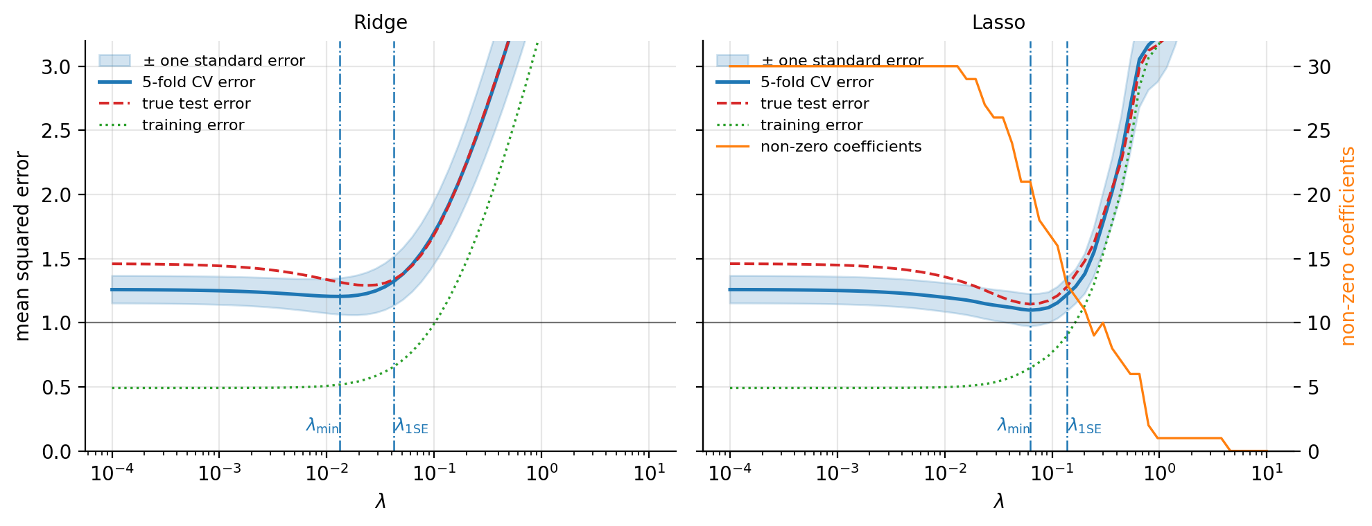
Figure 3.4: Five-fold cross-validation of Ridge (left) and the Lasso (right) on the sparse problem of the text: \(n=100\), \(p=30\), correlation \(0.7^{|i-j|}\), eight non-zero coefficients, \(\sigma=1\). The cross-validation error (3.92) is shown with its one-standard-error band (3.93); the dashed curve is the true expected test error of the model refitted at each \(\lambda\), measured on \(20\,000\) fresh observations, and the dotted curve the training error. The horizontal line is the noise floor \(\sigma^{2}=1\). The vertical lines mark \(\lambda_{\min}\) of Eq. (3.94) and \(\lambda_{1\mathrm{SE}}\) of Eq. (3.96); for the Lasso the number of non-zero coefficients is drawn against the right-hand axis.
The four test errors in the output deserve a comment of their own, because they illustrate a point that is easy to forget. They range from \(1.06\) to \(1.37\) and would seem to say that the one-standard-error Ridge beats the minimum-CV Ridge by a wide margin. They say no such thing. A mean squared error computed from \(50\) residuals is itself an estimate, and for Gaussian residuals its standard error is about \(\mathrm{MSE}\sqrt{2/50}\approx0.2\) (the squared residuals have variance \(2\,\mathrm{MSE}^{2}\), and Eq. (2.24) does the rest). The honest summary of the last column is that all four models generalise with an error of about \(1.2\pm0.2\), in agreement with their cross-validation estimates and above the floor of \(1\), and that a test set of fifty points cannot resolve differences of a tenth. The true errors quoted above, which can resolve them, were available only because we wrote the generating process ourselves.
Two further remarks on the cross-validation curves. First, the curve in the left panel lies below the true error for small \(\lambda\), by about \(0.2\). Cross-validation is if anything pessimistic – its models are fitted to \(80\) points rather than \(100\) – so this is not a systematic effect but the fluctuation of a single training set, of the size the standard error suggests; the repeated experiment later in this section will put a number on it. Second, the flatness of the curves near the minimum has a consequence for the selected penalty. Repeating the five-fold procedure with twenty different shuffles of the same training data,
for name, fit in (("Ridge", ridge_fit), ("Lasso", lasso_fit)):
    selected = [select(lambdas, *cv_curve(fit, X_train, y_train, lambdas, K=5,
                                          rng=np.random.default_rng(seed)))[0]
                for seed in range(20)]
    print(f"{name}: lambda_min over 20 shuffles between"
          f" {min(selected):.4f} and {max(selected):.4f}")
Ridge: lambda_min over 20 shuffles between 0.0028 and 0.0131
Lasso: lambda_min over 20 shuffles between 0.0050 and 0.0626
moves \(\lambda_{\min}\) by a factor of five for Ridge and by more than an order of magnitude for the Lasso. Read against the dashed curves of Figure 3.4, the Ridge choices all lie on the flat part and cost between nothing and a tenth in true error; the Lasso choices span true errors from \(1.15\) to \(1.41\) and retain anywhere between \(21\) and all \(30\) coefficients. The penalty selected from a single five-fold split is, in other words, a noisy quantity, and the Lasso’s support inherits the noise. Repeated cross-validation, which averages the curves over several shuffles before taking the minimum, reduces the wandering at a proportional cost; the one-standard-error rule is the cheaper remedy, since it moves the choice off the flat part and onto the rising flank, where the curve determines its own position; and the bootstrap experiment at the end of the section is the way to see how much of the selected support to trust.
The same procedure with scikit-learn.
Once the mechanics are understood, the library does the bookkeeping. A
Pipeline refits the scaler inside every fold, GridSearchCV
runs the loop over folds and penalties, and with refit=True it ends
by fitting the whole pipeline on all training data at the selected value.
The folds are passed explicitly so that they coincide with those of the code
above, and alpha is set to \(n_{\mathrm{fold}}\lambda=80\lambda\) so
that, inside the folds, Ridge solves exactly
Eq. (3.95).
from sklearn.linear_model import Ridge
from sklearn.model_selection import GridSearchCV
from sklearn.pipeline import Pipeline
from sklearn.preprocessing import StandardScaler

folds = np.array_split(np.random.default_rng(2024).permutation(100), 5)
cv = [(np.setdiff1d(np.arange(100), f), f) for f in folds]  # the same folds as above

model = Pipeline([("scale", StandardScaler()), ("ridge", Ridge())])
# scikit-learn's Ridge minimises ||y - X theta||^2 + alpha ||theta||^2, so
# alpha = n lambda, with n = 80 the size of the training folds
search = GridSearchCV(model, {"ridge__alpha": 80 * lambdas},
                      scoring="neg_mean_squared_error", cv=cv, refit=True)
search.fit(X_train, y_train)

lambda_star = search.best_params_["ridge__alpha"] / 80
cv_curve_sklearn = -search.cv_results_["mean_test_score"]
final_model = search.best_estimator_    # a new fit on all of X_train, not a fold fit
print(f"lambda* {lambda_star:.4f}, CV {-search.best_score_:.3f}, "
      f"test {np.mean((y_test - final_model.predict(X_test)) ** 2):.3f}")
cv_mean, _ = cv_curve(ridge_fit, X_train, y_train, lambdas, K=5,
                      rng=np.random.default_rng(2024))
print("largest difference from the hand-written curve:",
      np.max(np.abs(cv_curve_sklearn - cv_mean)))
lambda* 0.0131, CV 1.205, test 1.422
largest difference from the hand-written curve: 1.7763568394002505e-15
The two cross-validation curves agree to rounding error, which is the check
one should always make before trusting a library with a convention. The
test error does not agree – \(1.422\) against \(1.374\) from the hand-written
refit – and the reason is the factor \(n\) once more, now acting on the
refit: GridSearchCV refits with the same alpha\(=80\lambda^{\ast}\)
on all \(100\) observations, which in the per-observation convention is a
penalty of \(0.8\lambda^{\ast}\), and the final model is therefore slightly
less regularised than the one selected. Setting alpha to
\(100\lambda\) instead makes the refit exact but applies the full-sample
conversion inside \(80\)-point folds, which moves the selected value one grid
point, to \(0.0108\), with the cross-validation error unchanged in the third
decimal. Neither discrepancy matters here, both being a fraction of a grid
step on a flat curve, but both are the factor-\(n\) effect described above,
and knowing where it enters is what allows one to say so. Letting KFold(5, shuffle=True, random_state=2024)
choose its own folds instead of ours moves it much further, to
\(\lambda^{\ast}=0.0034\) with a cross-validation error of \(1.00\): the
wandering of the minimum along a flat valley again, and a reminder that
the second decimal of \(\lambda_{\min}\) is not a property of the data.
Leave-one-out and generalised cross-validation, revisited. For Ridge regression Section Statistical properties of the least-squares estimator derived the leave-one-out error in closed form, Eq. (3.40), and its rotation-invariant relative GCV, Eq. (3.41), both at the price of a single fit per \(\lambda\). When they apply they are excellent, and for small \(n\) they are the natural choice. Two things limit them. Their cost is that of forming the \(n\times n\) smoother matrix, which for large \(n\) exceeds that of \(K\) fits; and, more fundamentally, they require the fitted values to be a linear function of \(\bm{y}\). The Lasso fails this test: which coefficients are non-zero depends on \(\bm{y}\), so \(\tilde{\bm{y}}\) is piecewise linear in \(\bm{y}\) and no smoother matrix exists. (There is a remarkable partial substitute – the number of non-zero coefficients is an unbiased estimate of the Lasso’s effective degrees of freedom, so a GCV-like criterion can be written down – but it is not standard practice.) For the Lasso, and for every method in the later chapters of this book, \(K\)-fold cross-validation is the tool, and it is as well to learn it on a problem where its answer can be checked.
The bootstrap as an alternative.
Section The bias-variance tradeoff used the bootstrap of Section Resampling: the jackknife and the bootstrap to manufacture the ensemble of training sets that the bias-variance decomposition requires, and it is natural to ask whether the same device could estimate the test error and so replace cross-validation in the selection of \(\lambda\). It can be made to, and the care this takes is instructive, so we go through it.
Start with a fact about resampling with replacement. Each of the \(n\) draws picks observation \(i\) with probability \(1/n\), so the probability that \(i\) appears in none of them is
already \(0.366\) at \(n=100\). A bootstrap sample therefore contains, on average, only \(63.2\%\) of the distinct observations, the remainder appearing as duplicates; the \(36.8\%\) left out are the out-of-bag observations of the replica. This number governs everything that follows.
Three estimates of the prediction error can be built from bootstrap replicas. The apparent error is the training error \(\overline{\mathrm{err}}\) of the model fitted to the full sample; it is optimistic for the reasons of Section Statistical properties of the least-squares estimator and needs no bootstrap at all. The naive bootstrap estimate – fit to each replica, evaluate on the original \(n\) observations, average – is nearly as optimistic, because \(63\%\) of the observations it is evaluated on were in the sample it was fitted to. The estimate that respects the training-test separation is the leave-one-out bootstrap,
where \(C_{-i}\) is the set of replicas in which observation \(i\) does not appear and \(\hat{f}^{*b}\) is the model fitted to replica \(b\): every observation is predicted only by models that never saw it, exactly as in cross-validation. But each of those models was fitted to about \(0.632n\) distinct points, so Eq. (3.98) estimates the error of a model trained on a substantially smaller sample and is pessimistic. In terms of Eq. (3.92) it behaves like \(K\)-fold cross-validation with \((K-1)/K=0.632\), that is \(K\approx2.7\), whereas five folds train on \(80\%\) of the data and ten on \(90\%\). Efron’s remedy is to average the two biases away against each other,
the .632 estimator, whose weights are those of Eq. (3.97). It is a heuristic rather than a theorem, and it has a known failure: for a model that interpolates its training data, \(\overline{\mathrm{err}}=0\) and Eq. (3.99) returns \(0.632\) of a pessimistic number, which can be badly optimistic. The .632+ estimator repairs this by making the weight depend on an estimate of the degree of overfitting, at the price of further heuristics.
The following code computes the three bootstrap quantities for the problem of Figure 3.4, at the OLS end of the grid and at the two selected penalties, and sets them beside the five-fold estimate and the true error.
def bootstrap_errors(fit, X, y, lmbda, B=200, rng=None):
    """Training (apparent) error, leave-one-out bootstrap error, .632 estimate."""
    rng = np.random.default_rng() if rng is None else rng
    n = X.shape[0]
    theta_0, theta = refit(fit, X, y, lmbda)
    apparent = np.mean((y - theta_0 - X @ theta) ** 2)
    err_sum, err_count = np.zeros(n), np.zeros(n)
    for _ in range(B):
        idx = rng.integers(0, n, n)                         # draw n with replacement
        out = np.setdiff1d(np.arange(n), idx)               # the points left out
        theta_0, theta = refit(fit, X[idx], y[idx], lmbda)
        err_sum[out] += (y[out] - theta_0 - X[out] @ theta) ** 2
        err_count[out] += 1
    seen = err_count > 0
    loo_boot = np.mean(err_sum[seen] / err_count[seen])    # Eq. (3.loobootstrap)
    return apparent, loo_boot, 0.368 * apparent + 0.632 * loo_boot

rng = np.random.default_rng(3155)
X, y, theta_true = make_data(n=150, p=30, rho=0.7, sigma=1.0, rng=rng)
X_train, y_train = X[:100], y[:100]
# The generating process is known, so the true error of any fit can be measured
# on a large fresh sample -- a luxury never available in practice.
X_big, y_big, _ = make_data(n=20000, p=30, rho=0.7, sigma=1.0,
                            rng=np.random.default_rng(1))
lambdas = np.logspace(-4, 1, 60)

for name, fit in (("Ridge", ridge_fit), ("Lasso", lasso_fit)):
    cv_mean, cv_se = cv_curve(fit, X_train, y_train, lambdas, K=5,
                              rng=np.random.default_rng(2024))
    lambda_min, lambda_1se = select(lambdas, cv_mean, cv_se)
    for lmbda in (1e-4, lambda_min, lambda_1se):
        j = np.searchsorted(lambdas, lmbda)
        apparent, loo_boot, e632 = bootstrap_errors(fit, X_train, y_train, lmbda,
                                                    B=200, rng=np.random.default_rng(2024))
        theta_0, theta = refit(fit, X_train, y_train, lmbda)
        true = np.mean((y_big - theta_0 - X_big @ theta) ** 2)
        print(f"{name} lambda {lmbda:.4f}: train {apparent:.3f}  CV {cv_mean[j]:.3f}"
              f"  LOO-boot {loo_boot:.3f}  .632 {e632:.3f}  true {true:.3f}")

# When p approaches n the bootstrap training sets, with only 0.632 n distinct
# points, reach the singular regime of the Franke study long before the K-fold ones
rng = np.random.default_rng(5)
X, y, _ = make_data(n=100, p=60, rho=0.7, sigma=1.0, rng=rng)
X_big, y_big, _ = make_data(n=20000, p=60, rho=0.7, sigma=1.0,
                            rng=np.random.default_rng(6))
apparent, loo_boot, e632 = bootstrap_errors(ridge_fit, X, y, 1e-4, B=200, rng=rng)
cv_mean, _ = cv_curve(ridge_fit, X, y, np.array([1e-4]), K=5, rng=rng)
theta_0, theta = refit(ridge_fit, X, y, 1e-4)
print(f"p = 60, n = 100, lambda 0.0001: train {apparent:.3f}  CV {cv_mean[0]:.3f}"
      f"  LOO-boot {loo_boot:.3f}  .632 {e632:.3f}"
      f"  true {np.mean((y_big - theta_0 - X_big @ theta) ** 2):.3f}")
Ridge lambda 0.0001: train 0.491  CV 1.258  LOO-boot 1.476  .632 1.114  true 1.459
Ridge lambda 0.0131: train 0.517  CV 1.205  LOO-boot 1.409  .632 1.080  true 1.316
Ridge lambda 0.0424: train 0.659  CV 1.324  LOO-boot 1.647  .632 1.284  true 1.338
Lasso lambda 0.0001: train 0.491  CV 1.258  LOO-boot 1.476  .632 1.114  true 1.460
Lasso lambda 0.0626: train 0.648  CV 1.098  LOO-boot 1.286  .632 1.051  true 1.145
Lasso lambda 0.1366: train 0.896  CV 1.216  LOO-boot 1.526  .632 1.294  true 1.277
p = 60, n = 100, lambda 0.0001: train 0.480  CV 5.088  LOO-boot 24.969  .632 15.957  true 3.255
The pattern predicted above is the pattern observed. The training error is optimistic by a factor of up to three; the leave-one-out bootstrap is pessimistic at every penalty, by an amount that grows with \(\lambda\) and reaches \(0.3\); the .632 estimator lands between them, on this training set below the truth at the smaller penalties by up to \(0.35\); and the five-fold estimate is within one to one and a half of its own standard errors of the truth at every penalty. Figure 3.5 shows the same four estimates along the whole grid, with the true curve, and marks the minimum of each. The last line of the output is the case where the difference stops being a matter of tenths. With \(p=60\) features and \(n=100\) observations the five-fold models, fitted to \(80\) points, are still comfortably overdetermined, and cross-validation overestimates the true error of \(3.3\) by a factor of \(1.5\) – pessimistic, as models trained on fewer points must be near the \(p\approx n\) cliff of Section A complete example: the Franke function. The bootstrap models are fitted to about \(63\) distinct points, right at the edge of that cliff, and their out-of-bag error is \(25\); the .632 correction brings it down to \(16\), still five times the truth. Duplicated rows make the matter worse than the count of distinct points suggests: a replica is a weighted least-squares problem with integer weights, so its design matrix has the column space of the \(63\) distinct rows but a distorted geometry, and for the Lasso the duplicates change which variables enter.
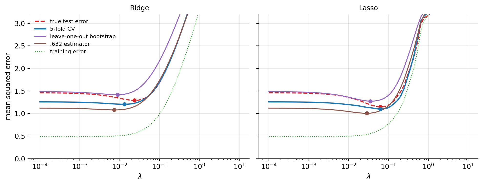
Figure 3.5: Four estimates of the test error of Ridge (left) and the Lasso (right) along the penalty grid, for the training set of Figure 3.4: the training error, five-fold cross-validation (3.92), the leave-one-out bootstrap (3.98) and the .632 estimator (3.99), with \(B=100\) replicas per grid point. The dashed curve is the true expected test error. Dots mark the minimum of each curve: the .632 minimum sits to the left of the true one because the estimator inherits \(0.368\) of the training error, which decreases towards \(\lambda=0\).
A single training set cannot separate bias from luck, so we repeat the comparison over a hundred fresh training sets at a fixed penalty and record, for each estimator, the mean and the spread of its deviation from the true error of the model it is estimating.
X_big, y_big, _ = make_data(n=20000, p=30, rho=0.7, sigma=1.0,
                            rng=np.random.default_rng(1))
# bias and spread of the four estimators over 100 fresh training sets, at fixed lambda
for name, fit, lmbda in (("Ridge", ridge_fit, 0.0131), ("Lasso", lasso_fit, 0.0626)):
    rows = []
    for seed in range(100):
        rng = np.random.default_rng(100 + seed)
        X, y, _ = make_data(n=100, p=30, rho=0.7, sigma=1.0, rng=rng)
        cv_mean, _ = cv_curve(fit, X, y, np.array([lmbda]), K=5, rng=rng)
        apparent, loo_boot, e632 = bootstrap_errors(fit, X, y, lmbda, B=100, rng=rng)
        theta_0, theta = refit(fit, X, y, lmbda)
        true = np.mean((y_big - theta_0 - X_big @ theta) ** 2)
        rows.append((apparent, cv_mean[0], loo_boot, e632, true))
    rows = np.array(rows)
    deviation = rows[:, :4] - rows[:, 4:5]                 # estimate minus true error
    print(f"{name} at lambda = {lmbda}: mean true error {rows[:, 4].mean():.3f}")
    print("  bias (training, CV, LOO-bootstrap, .632):", np.round(deviation.mean(0), 3))
    print("  spread                                 :", np.round(deviation.std(0), 3))
Ridge at lambda = 0.0131: mean true error 1.444
  bias (training, CV, LOO-bootstrap, .632): [-0.737  0.137  0.477  0.03 ]
  spread                                 : [0.165 0.346 0.323 0.259]
Lasso at lambda = 0.0626: mean true error 1.327
  bias (training, CV, LOO-bootstrap, .632): [-0.532  0.055  0.287 -0.014]
  spread                                 : [0.164 0.274 0.267 0.225]
The biases are as advertised: the training error is optimistic by half a unit or more, the leave-one-out bootstrap pessimistic by \(0.3\) to \(0.5\), and five-fold cross-validation pessimistic by \(0.05\) to \(0.14\), which is the price of fitting to \(80\) points instead of \(100\) and shrinks as \(K\) grows. The gap of \(0.2\) noticed in Figure 3.4 was, as claimed, a fluctuation, of about one spread. What the table also shows, and what an honest account must say, is that at a fixed penalty the .632 estimator is the best of the four: nearly unbiased, and with a spread smaller than that of cross-validation by a fifth to a quarter. This is Efron and Tibshirani’s finding and it is not a coincidence – averaging over \(B\) replicas is a smoother operation than averaging over five folds. If the question were “what is the test error of this model at this \(\lambda\)”, the bootstrap would have a strong claim.
That is not the question. The question is which \(\lambda\) to choose, and for that purpose cross-validation is preferred for four reasons which the experiments above have made concrete. First, selection depends on the location of the minimum, not on the level of the curve. A bias that is nearly constant in \(\lambda\), which is what cross-validation has, leaves the minimum where it is; the .632 estimator adds \(0.368\) of the training error, a function that decreases monotonically towards \(\lambda=0\), and its minimum is thereby dragged towards under-regularisation. In Figure 3.5 it selects \(0.007\) for Ridge and \(0.029\) for the Lasso, against true optima of \(0.024\) and \(0.063\) and cross-validation choices of \(0.013\) and \(0.063\); for the Lasso the .632 choice keeps \(26\) coefficients where cross-validation keeps \(21\). Second, cost: five or ten fits per grid point against one or two hundred, which for the sixty-point grid above is three hundred fits against twelve thousand, and the ratio is the same for a neural network taking an hour per fit. Third, sample size: the bootstrap models see \(63\%\) of the distinct data and fall off the \(p\approx n\) cliff first, as the last line of the table shows, while \(K\)-fold models see \((K-1)/K\) of it and can be pushed as close to the full sample as one is willing to pay for. Fourth, simplicity: every observation is predicted exactly once, by a model that did not see it, from a training set of the same character as the final one, and no correction constants are needed – whereas the bootstrap estimate requires the .632 heuristic, and the .632 heuristic requires the .632+ repair as soon as the apparent error approaches zero, which for \(p\ge n\) it does.
What the bootstrap is for: the stability of the selection.
None of this retires the bootstrap. It remains the tool for estimating the distribution of a statistic when no formula exists, which is how Chapter 2 used it, and cross-validation produces a statistic to which no formula applies: the set of coefficients the Lasso selects. The output above found \(21\) non-zero coefficients at \(\lambda_{\min}\), eight true and thirteen spurious, and nothing in the cross-validation curve says which are which. The bootstrap can. Refit the Lasso, at the selected penalty, to \(B\) replicas of the training set and record how often each coefficient is non-zero:
cv_mean, cv_se = cv_curve(lasso_fit, X_train, y_train, lambdas, K=5,
                          rng=np.random.default_rng(2024))
lambda_min, _ = select(lambdas, cv_mean, cv_se)

# selection frequency of every feature over B bootstrap replicas at lambda_min
rng, B, n = np.random.default_rng(2024), 200, 100
count = np.zeros(X_train.shape[1])
for _ in range(B):
    idx = rng.integers(0, n, n)
    theta_0, theta = refit(lasso_fit, X_train[idx], y_train[idx], lambda_min)
    count += theta != 0
frequency = count / B
theta_0, theta = refit(lasso_fit, X_train, y_train, lambda_min)
print("selected on the full training set:", np.flatnonzero(theta))
print("frequency, the eight true features:", np.round(frequency[:8], 2))
print("frequency, the spurious ones selected:")
print(np.round(frequency[8:][theta[8:] != 0], 2))
print("selected in more than 80% of the replicas:", np.flatnonzero(frequency > 0.8))
selected on the full training set: [ 0  1  2  3  4  5  6  7 10 12 13 14 16 17 20 23 24 26 27 28 29]
frequency, the eight true features: [1.   1.   1.   1.   1.   1.   0.97 1.  ]
frequency, the spurious ones selected:
[0.64 0.74 0.78 0.72 0.53 0.68 0.56 0.64 0.86 0.75 0.61 0.51 0.82]
selected in more than 80% of the replicas: [ 0  1  2  3  4  5  6  7 24 29]
The eight true features are selected in \(97\) to \(100\) per cent of the replicas; the thirteen spurious ones in \(51\) to \(86\) per cent, most of them in around two thirds. A coefficient that appears in two replicas out of three is one whose presence depends on which observations happened to be drawn, and that is the operational meaning of “spurious” when the truth is unknown. Keeping only the features selected in more than \(80\%\) of the replicas leaves the eight true ones and two impostors, which is a far better support than the \(21\) the cross-validation minimum returned – and it was obtained without the one-standard-error rule, without knowing the truth, and without any estimate of the test error at all. This procedure, refined and supplied with an error bound on the number of false selections, is stability selection, and it is the natural companion to a cross-validated Lasso: cross-validation chooses the penalty for prediction, and the bootstrap tells us which parts of the resulting model to believe. The same replicas can be used to attach a standard error to every non-zero coefficient, to the cross-validation curve itself, and to \(\lambda_{\min}\), which is how the wandering reported earlier would be quantified in practice.
Nested cross-validation.
One question remains, and it is the one the test set answered above: what is the generalisation error of the whole procedure, selection included? The temptation is to report \(\mathrm{CV}_K(\lambda_{\min})\), the smallest value on the curve, and it is a mistake, for the same reason that the training error is a mistake one level down. The minimum of sixty noisy estimates is biased downwards – among sixty candidates, the one with the luckiest noise wins – and the more penalties one tries, the larger the effect. With a test set the question does not arise: the test error of the refitted model is an unbiased estimate of exactly the right thing. Without one, the remedy is to nest the selection inside a second cross-validation loop: an outer split into \(K_{\mathrm{out}}\) folds, and within each outer training set the full inner procedure – grid, \(K\) folds, selection, refit – followed by evaluation on the outer held-out fold. Every outer fold then tests a model whose \(\lambda\) was chosen without it, the outer average estimates the error of the procedure rather than of a particular \(\lambda\), and the cost is \(K_{\mathrm{out}}\) times that of the inner loop. For the linear models of this chapter the cost is negligible and the selection bias is small – the cross-validation minimum of \(1.10\) for the Lasso above sits below the true \(1.15\) by an amount well inside the noise – but for flexible models with several hyperparameters tuned on a fine grid it is neither, and nested cross-validation is the honest estimate.
Machine learning connection
The procedure of this section is not specific to \(\lambda\). Every method in the remainder of this book has hyperparameters – the learning rate and batch size of Chapter 4, the depth of a tree, the kernel width of Chapter 6, the width and depth of a network – and none of them can be chosen by minimising the training error, for the reason of Eq. (3.91): a more flexible model always fits the training data better. They are all chosen the way \(\lambda\) was chosen here, by cross-validation on the training data, with the preprocessing inside the loop, with a refit at the selected values, and with the test set used exactly once afterwards. Two things change as the models grow. The cost of a fit grows, which is why one sees \(K=3\) and single validation splits in deep learning where this chapter used \(K=5\) and could have afforded leave-one-out; and the number of hyperparameters grows, so that the grid becomes a random or adaptive search over a space rather than a line, and the selection bias that nested cross-validation guards against becomes real. The discipline is the same. Cross-validation chooses the hyperparameters; refitting produces the final parameters; the test set is a test set only as long as it has been used once.
3.15. A complete example: the Franke function#
We now assemble everything into a single study. The Franke function is a weighted sum of four exponentials on the unit square,
for \(x,y\in[0,1]\). It is a standard test surface for interpolation and regression: smooth, but with two peaks, a saddle and a depression, so that it cannot be captured by a low-order polynomial and is well captured by a moderate one. Adding Gaussian noise gives us a problem with a known truth, a known noise level and a tunable complexity – everything needed to see the bias-variance trade-off of Section The bias-variance tradeoff in action.
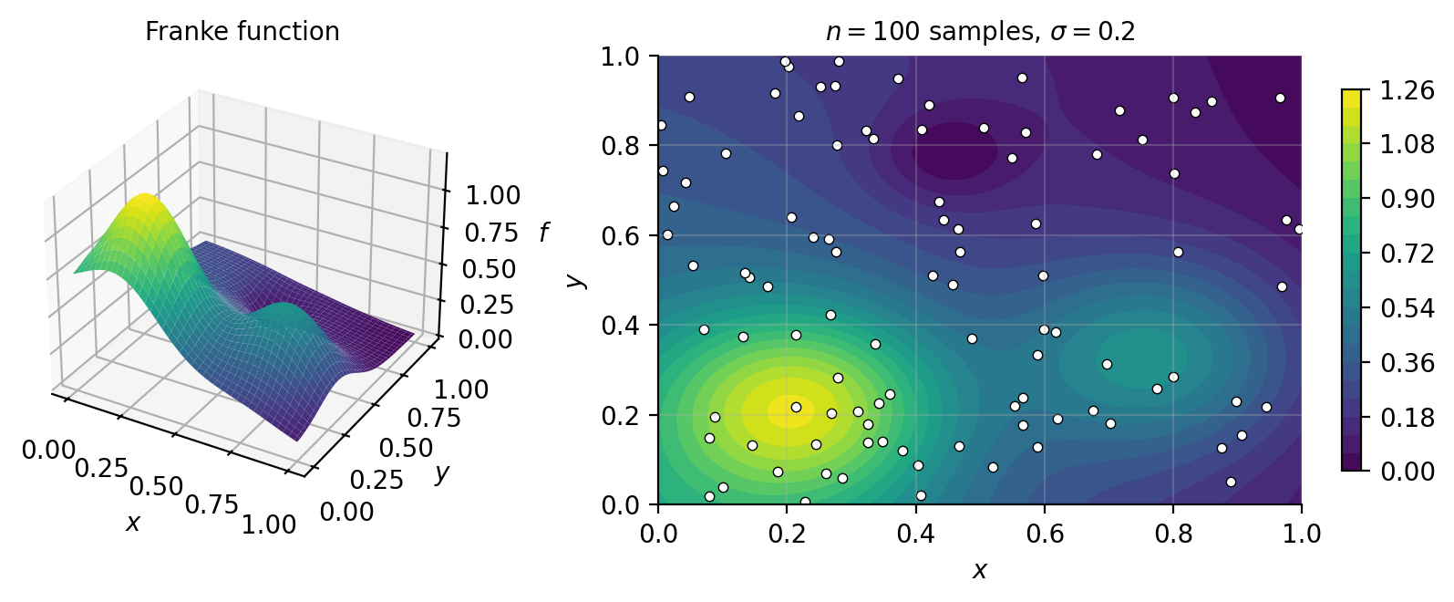
Figure 3.6: The Franke function (3.100) on the unit square (left) and a contour view with the \(n=100\) noisy samples used in this section marked (right). Two peaks, a saddle and a depression make it too rich for a low-order polynomial and well within reach of a moderate one.
import numpy as np

def franke_function(x, y):
    """The Franke function, Eq. (3.franke)."""
    t1 = 0.75 * np.exp(-(0.25 * (9 * x - 2)**2) - 0.25 * ((9 * y - 2)**2))
    t2 = 0.75 * np.exp(-((9 * x + 1)**2) / 49.0 - 0.1 * (9 * y + 1))
    t3 = 0.50 * np.exp(-(9 * x - 7)**2 / 4.0 - 0.25 * ((9 * y - 3)**2))
    t4 = -0.20 * np.exp(-(9 * x - 4)**2 - (9 * y - 7)**2)
    return t1 + t2 + t3 + t4


def make_franke_data(n=400, noise=0.1, rng=None):
    """Sample the Franke function on random points with Gaussian noise."""
    rng = np.random.default_rng() if rng is None else rng
    x, y = rng.random(n), rng.random(n)
    z = franke_function(x, y) + noise * rng.normal(size=n)
    return x, y, z
The study. The analysis proceeds in the order of this book. We build the design matrix of Eq. (3.5) for polynomial degrees from one to some maximum; we split the data into training and test sets; we standardise using training statistics only; we fit by OLS, Ridge and Lasso; and we report test errors, choosing \(\lambda\) by the \(k\)-fold cross-validation of Section Choosing the penalty: cross-validation for Ridge and Lasso, with the scaler refitted inside every fold and the model refitted on the full training set at the selected value.
import numpy as np
from sklearn.linear_model import LinearRegression, Ridge, Lasso
from sklearn.preprocessing import StandardScaler
from sklearn.pipeline import make_pipeline
from sklearn.model_selection import train_test_split, KFold, cross_val_score

rng = np.random.default_rng(2024)
# A small, noisy sample: with n = 100 the number of parameters (3.numfeatures)
# overtakes the 80 training points around degree eleven, which is where the
# difference between the three methods becomes visible.
x, y, z = make_franke_data(n=100, noise=0.2, rng=rng)

max_degree = 14
kfold = KFold(n_splits=5, shuffle=True, random_state=2024)
lambdas = np.logspace(-5, 1, 25)

results = {"OLS": [], "Ridge": [], "Lasso": []}
for degree in range(1, max_degree + 1):
    X = design_matrix_2d(x, y, degree)[:, 1:]      # drop the intercept column
    X_train, X_test, z_train, z_test = train_test_split(X, z, test_size=0.2,
                                                        random_state=2024)

    # OLS: the scaler is fitted on the training fold only, inside the pipeline
    ols_pipe = make_pipeline(StandardScaler(), LinearRegression())
    ols_pipe.fit(X_train, z_train)
    results["OLS"].append(mse(z_test, ols_pipe.predict(X_test)))

    # Ridge and Lasso: choose lambda by cross-validation on the training set
    for name, Model in (("Ridge", Ridge), ("Lasso", Lasso)):
        cv_error = [
            -cross_val_score(make_pipeline(StandardScaler(),
                                           Model(alpha=lmb, max_iter=5000)),
                             X_train, z_train, cv=kfold,
                             scoring="neg_mean_squared_error").mean()
            for lmb in lambdas
        ]
        best = make_pipeline(StandardScaler(),
                             Model(alpha=lambdas[int(np.argmin(cv_error))],
                                   max_iter=5000))
        best.fit(X_train, z_train)
        results[name].append(mse(z_test, best.predict(X_test)))
        if name == "Lasso":
            n_kept = int(np.sum(best[-1].coef_ != 0))

for name, errors in results.items():
    print(f"{name:>6}: best degree {int(np.argmin(errors)) + 1:2d}, "
          f"test MSE {min(errors):.4f}, "
          f"MSE at degree {max_degree} {errors[-1]:.4f}")
What one observes. The output of the run above is
   OLS: best degree  4, test MSE 0.0570, MSE at degree 14 2428714.9322
 Ridge: best degree  2, test MSE 0.0599, MSE at degree 14       0.0667
 Lasso: best degree  3, test MSE 0.0607, MSE at degree 14       0.0644
and three features of it are worth dwelling on, because they are the lessons of the preceding chapters made visible.
First, all three methods achieve very nearly the same best test error, about \(0.057\) to \(0.061\), against a noise variance of \(\sigma^{2}=0.04\). By Eq. (2.52) that floor cannot be crossed, and the three methods are all within about fifty per cent of it. Regularisation does not make a good model better.
Second, the behaviour away from the optimum is entirely different. The OLS error is well behaved up to degree eight, rises to \(14.5\) at degree ten and then to over two million at degree fourteen – seven orders of magnitude worse than its own best value. The reason is Eq. (3.5): at degree fourteen there are \(119\) parameters and only \(80\) training points, so \(\bm{X}^{T}\bm{X}\) is singular, the smallest singular values are pure noise, and Eq. (3.11) divides by them. The penalised errors, by contrast, rise from \(0.060\) to \(0.067\) and from \(0.061\) to \(0.064\): they barely move. Cross-validation increases \(\lambda\) as the degree grows, and the shrinkage factors (3.48) suppress precisely the directions in which Eq. (3.42) shows the variance to be unbounded. What regularisation buys is not a better optimum but insensitivity to choosing the complexity badly – which matters, because in a real problem the right complexity is not known.
Third, the Lasso fits are genuinely sparse. At degree ten it keeps \(6\) of \(65\) coefficients, and at degree fourteen \(7\) of \(119\); Ridge at comparable test error keeps every one of them, each small. The Lasso has performed model selection, discovering from the data that a handful of low-order monomials suffices – consistent with its optimum at degree three.
Two further experiments make the point sharper. Increasing \(n\) from \(100\) to \(400\) moves the OLS optimum from degree four to degree eleven and reduces the degradation at degree fourteen from a factor of \(4\times10^{7}\) to a factor of \(3\), because \(p\) no longer approaches \(n\). Reducing the noise to \(\sigma=0\) while keeping \(n=100\) moves the optimum from degree four to degree eight, since with no noise there is less to overfit. Note that even then the error eventually grows, by a factor of about \(180\) at degree fourteen: once \(p\) exceeds the number of training points the design matrix is rank deficient and Eq. (3.11) is dividing by singular values that are pure rounding error. That failure is one of conditioning rather than of statistics, and it is the only one of the three that no amount of clean data will cure. The best model is a property of the data set – its size and its noise level – and not of the function being approximated.
Figure 3.7 presents the whole experiment at a glance. The left panel is the test error, on a logarithmic scale so that the seven orders of magnitude are visible at all; the right panel counts the coefficients the Lasso retains. Read together they make the argument of this chapter: all three methods reach the same floor, set by the irreducible \(\sigma^{2}\), but only the penalised ones stay near it when the complexity is chosen badly, and only the Lasso tells us how many terms were needed.
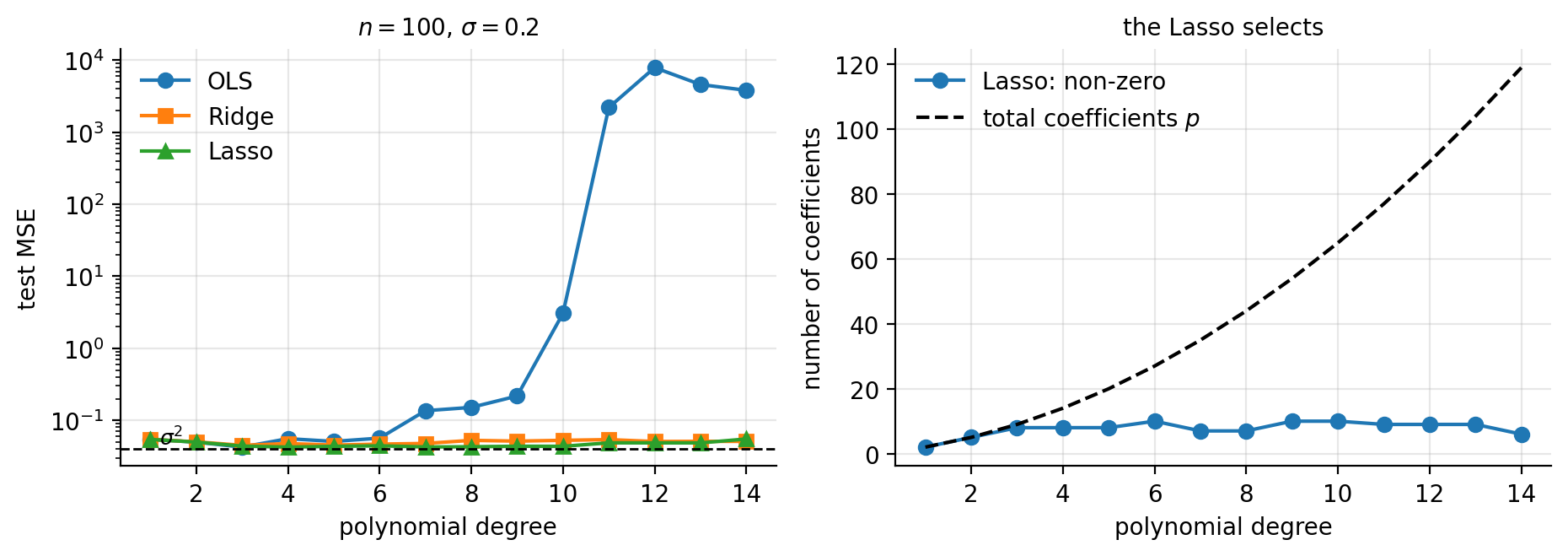
Figure 3.7: Test error against polynomial degree for the three estimators on the Franke data (left, logarithmic), with the noise floor \(\sigma^{2}=0.04\) marked; and the number of coefficients the Lasso retains against the total number available (right).
Machine learning connection
The whole analysis rests on one number being honest: the test error. It is worth listing the ways of corrupting it, all of which appear in student work and published papers alike. Standardising before the split leaks the test distribution into training. Choosing the polynomial degree by looking at the test error, then reporting that same error, turns the test set into a validation set – the reported figure is then optimistic, and the remedy is the three-way split of Section Training error, test error and generalisation. Selecting features on the full data set before cross-validating leaks in the same way, and dramatically so when \(p\) is large. And splitting spatially or temporally correlated data at random makes the test points near-duplicates of training points, which by Section Correlated data and the autocorrelation function measures interpolation rather than prediction. For data sampled on a grid, as the Franke function often is, this last is a real concern.
3.16. A second example: the one-dimensional Ising model#
The Franke function was a regression problem dressed as a surface. This section is a regression problem dressed as a piece of physics, and it is worth the detour for three reasons. The design matrix is singular exactly, by an amount we can count in advance, so it exhibits everything Section Ridge regression said about ill-conditioning without any appeal to rounding error. The three estimators return visibly different answers to the same question, and the differences are the ones the theory predicts rather than accidents of the solver. And the correct answer is known, so we can ask not only which estimator predicts well but which one is right.
3.16.1. The model and the design matrix#
Consider \(L\) classical spins \(s_j\in\{-1,+1\}\) arranged on a ring, with the nearest-neighbour Hamiltonian
This is the one-dimensional Ising model, and \(J>0\) favours aligned neighbours. Now forget that we know Eq. (3.101) and suppose instead that we are handed a pile of configurations \(\bm{s}^{(i)}\) together with their energies \(y_i=H(\bm{s}^{(i)})\), and are asked to discover the physics. A reasonable thing to assume is that the interaction is pairwise but otherwise unrestricted,
with an unknown coupling matrix \(\bm{J}\). The point of writing it this way is that Eq. (3.102) is linear in the unknowns: the \(L^{2}\) numbers \(J_{jk}\) enter multiplied by the observable products \(s_js_k\). Setting \(\theta_{jL+k}=-J_{jk}\) and
turns the problem into \(\bm{y}=\bm{X}\bm{\theta}\), an ordinary linear model with \(p=L^{2}\) features, and every tool of this chapter applies unchanged. The physics has been hidden inside the design matrix, which is exactly what the phrase feature engineering means.
import numpy as np

rng = np.random.default_rng(2718)
L, n, Jtrue = 40, 10000, 1.0
spins = rng.choice([-1, 1], size=(n, L))
energies = -Jtrue * np.einsum("ij,ij->i", spins, np.roll(spins, 1, axis=1))

# design matrix, Eq. (3.isingdesign): X[i, j*L+k] = s_j s_k
X = np.einsum("ij,ik->ijk", spins, spins).reshape(n, L * L)
There is a price for the convenience, and it is paid immediately. The design matrix (3.103) is not of full column rank, and not by a little.
Proposition 3.14 (The Ising design matrix is exactly rank deficient)
Let \(\bm{X}\) be given by Eq. (3.103) for spins \(s_j\in\{-1,+1\}\). Then
for every sample size \(n\), whereas the number of columns is \(L^{2}\).
Proof
Two families of columns coincide identically, whatever the configurations. First, the column indexed \((j,j)\) has entries \(\left(s_j^{(i)}\right)^{2}=1\) for every \(i\), since \(s_j\in\{-1,+1\}\); all \(L\) diagonal columns are therefore the constant column \(\bm{1}\) and equal to one another. Second, the columns indexed \((j,k)\) and \((k,j)\) have entries \(s_j s_k\) and \(s_k s_j\), which are the same number. So the \(L^{2}\) columns take at most \(L(L-1)/2+1\) distinct values: one for the diagonal, and one for each unordered pair \(j<k\). The rank cannot exceed the number of distinct columns. \qed
For \(L=40\) the bound is \(40\cdot39/2+1=781\) against \(p=1600\) columns, so more than half the columns are redundant by construction. This is worth pausing over. Section Ridge regression motivated the penalty by saying that \(\bm{X}^{T}\bm{X}\) becomes ill-conditioned when features are nearly collinear; here they are exactly collinear, and no amount of extra data can help, because the coincidences of the proof hold configuration by configuration. The program confirms both the identities and the bound:
  max |X[:, diagonal] - 1|                    : 0.000e+00
  max |X[:, (j,k)] - X[:, (k,j)]| over all j<k: 0.000e+00

  distinct columns therefore number L(L-1)/2 + 1 = 781,
  so rank(X) <= 781 however many configurations we draw.
  measured rank(X) with n = 10000 rows          : 781
  number of columns p = L^2                   : 1600
  singular values: sigma_0 = 633.8002, sigma_780 = 1.0218e+02, sigma_781 = 4.7516e-13
  ratio sigma_780 / sigma_781 : 2.150e+14
The bound is attained, and the singular value spectrum falls off a cliff exactly at index \(781\), dropping by fourteen orders of magnitude between one singular value and the next. Figure 3.8 shows it. In the expansion (3.11) the least-squares coefficient along each right singular vector is \(\bm{u}_i^{T}\bm{y}/\sigma_i\); here \(819\) of those denominators are zero, and the pseudoinverse of Section Ordinary least squares handles them by declaring the corresponding coefficients to be zero – the minimum-norm choice. That convention is about to have a visible physical consequence.
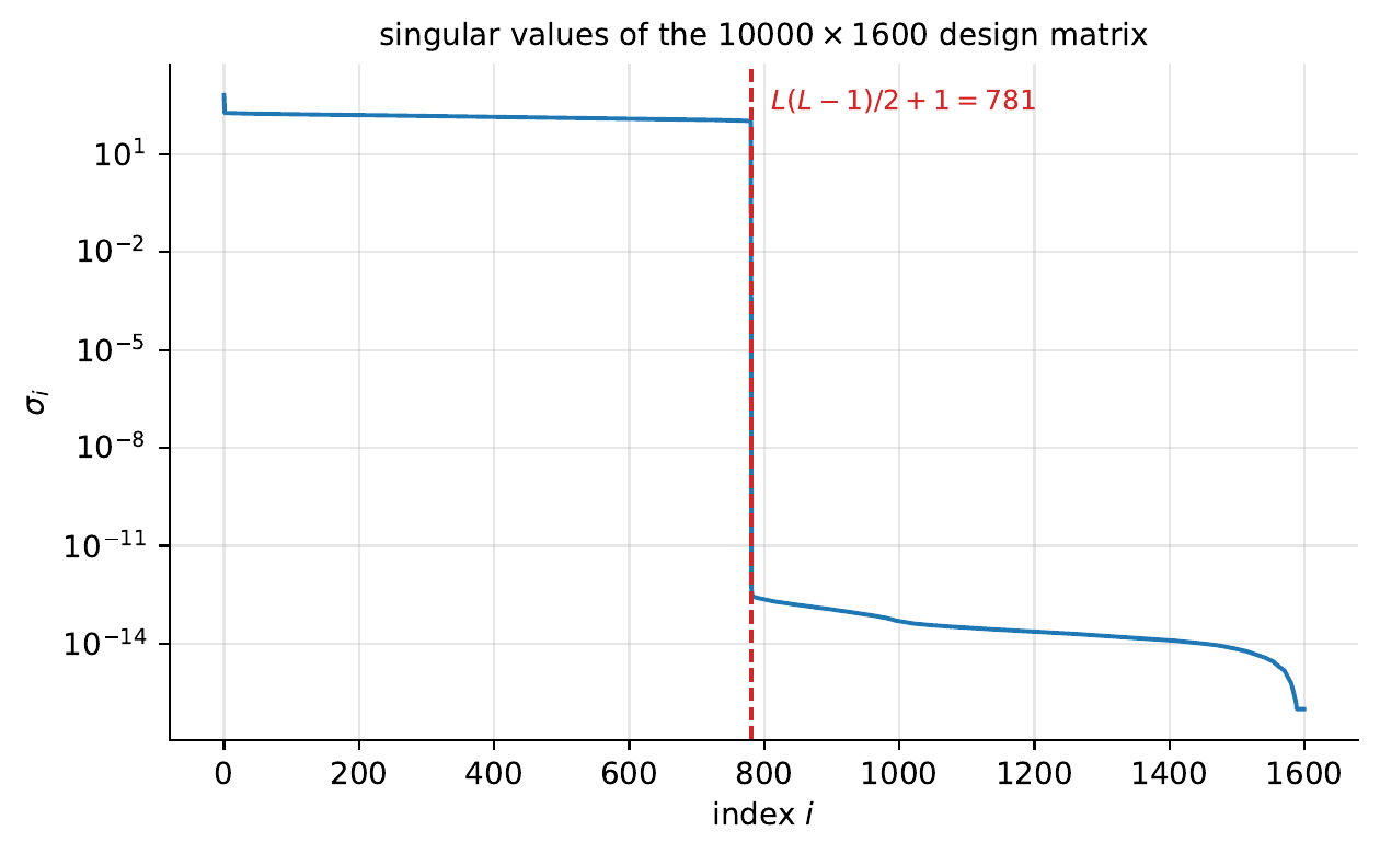
Figure 3.8: Singular values of the \(10000\times1600\) Ising design matrix (3.103) for \(L=40\). The spectrum collapses precisely at the index \(L(L-1)/2+1=781\) predicted by Proposition 3.14: the rank deficiency is a property of the features, not of the sample.
3.16.2. Fitting with \(p\) four times \(n\)#
We use \(n_{\mathrm{train}}=400\) configurations to fit \(p=1600\) coefficients and keep the remaining \(9600\) for testing. The problem is therefore underdetermined twice over: once because \(p>n\), and once more because of Proposition 3.14. Ridge regression is solved in the dual form of Theorem 3.11, which here means a \(400\times400\) system instead of a \(1600\times1600\) one, and the Lasso by the coordinate descent of Eq. (3.69).
   estimator            R^2 train  R^2 test  ||theta||_2  ||theta||_1  non-zero
   OLS (pseudoinverse)    1.000000  0.522863       3.2610      88.9391      1600
   Ridge, lambda = 0.01   1.000000  0.522863       3.2609      88.9379      1600
   Lasso, lambda = 0.01   0.999973  0.999963       6.1351      39.7766        78
Three things in one table. OLS reproduces the training energies exactly – with \(1600\) free parameters and \(400\) equations it could hardly fail – and then explains barely half the variance of the test set. Ridge at \(\lambda=10^{-2}\) is indistinguishable from OLS to four decimal places, which is not a bug and is discussed below. And the Lasso is essentially perfect on data it has never seen, using \(78\) of the \(1600\) coefficients.
The last number is the interesting one, because \(78=2\times39\) is very nearly \(2L=80\): the Lasso has found the nearest-neighbour couplings and almost nothing else. Figure 3.9 shows the three recovered coupling matrices, and the difference is not subtle.
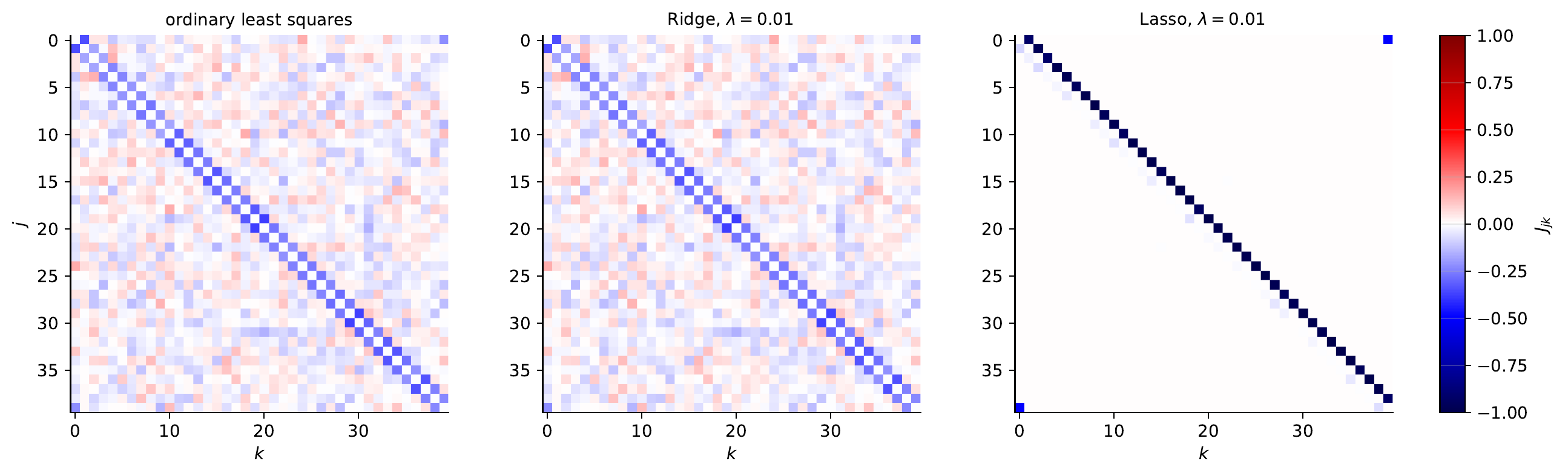
Figure 3.9: The coupling matrices \(J_{jk}\) recovered from \(400\) configurations of the \(L=40\) Ising chain. The truth is a single off-diagonal band. OLS and Ridge spread the interaction over the whole matrix and split each coupling symmetrically between \((j,k)\) and \((k,j)\); the Lasso finds the band and puts each coupling entirely on one side of the pair. Both behaviours are forced, by Proposition 3.15.
3.16.3. Why the symmetry, and why only for two of the three#
The pattern in Figure 3.9 is not a quirk of this data set. It is a theorem about duplicated columns, and it explains the behaviour of all three estimators at once.
Proposition 3.15 (Duplicated columns)
Suppose two columns of \(\bm{X}\) are identical, say columns \(a\) and \(b\). Then
the Ridge estimator (3.44) satisfies \(\hat\theta_a=\hat\theta_b\) for every \(\lambda>0\), and so does the minimum-norm least-squares solution (3.11);
the Lasso fit \(\bm{X}\hat{\bm{\theta}}\) is unique, but any redistribution of \(\hat\theta_a+\hat\theta_b\) between the two coefficients that keeps both of the same sign is also a minimiser.
Proof
Let \(P\) be the permutation that swaps coordinates \(a\) and \(b\). Because the two columns are equal, \(\bm{X}P=\bm{X}\), so the residual sum of squares obeys \(\mathrm{RSS}(P\bm{\theta})=\mathrm{RSS}(\bm{\theta})\); the \(2\)-norm satisfies \(\|P\bm{\theta}\|_2=\|\bm{\theta}\|_2\) as well, so the whole Ridge objective is invariant under \(P\). It is also strictly convex, hence has a unique minimiser \(\hat{\bm{\theta}}\), and \(P\hat{\bm{\theta}}\) is a minimiser too; uniqueness forces \(P\hat{\bm{\theta}}=\hat{\bm{\theta}}\), that is \(\hat\theta_a=\hat\theta_b\). For OLS the objective is invariant but not strictly convex; the minimum-norm solution is nevertheless unique, and the same argument applies to it because \(P\) preserves the norm being minimised.
For the Lasso, uniqueness of the fit is Proposition 3.9. Write \(t=\hat\theta_a+\hat\theta_b\) and replace \((\hat\theta_a,\hat\theta_b)\) by \((u,t-u)\). The residual depends only on \(t\), since the columns are equal, and if \(u\) and \(t-u\) share the sign of \(t\) then \(|u|+|t-u|=|t|\), so the penalty is unchanged as well. The objective is therefore constant along that whole segment. \qed
Applied here: the columns \((j,k)\) and \((k,j)\) are equal, so OLS and Ridge must report \(J_{jk}=J_{kj}\), and the physics – which only ever constrains the sum \(J_{jk}+J_{kj}\) – is split down the middle. The Lasso is under no such obligation, and the solver, sweeping the coordinates in order, arrives at a vertex of the optimal segment. Both statements are visible in the output:
   estimator              J[0,1]    J[1,0]       sum    J[0,0]    J[0,5]
   OLS (pseudoinverse)   -0.34863  -0.34863  -0.69726  -0.00490  -0.03488
   Ridge, lambda = 0.01  -0.34863  -0.34863  -0.69725  -0.00490  -0.03488
   Lasso, lambda = 0.01  -0.91691  -0.08149  -0.99840  -0.00000  -0.00000
   estimator            max |J[j,k] - J[k,j]| over all j<k
   OLS (pseudoinverse)                           9.437e-16
   Ridge, lambda = 0.01                          0.000e+00
   Lasso, lambda = 0.01                          9.990e-01
The \(2\)-norm estimators are symmetric to machine precision, as the proposition requires, and the Lasso is as asymmetric as it is possible to be, the two entries differing by very nearly the whole coupling. The sum, though, is \(-0.9984\) against a true value of \(-1\): what the data determine, the Lasso gets right. That the split is genuinely arbitrary can be checked directly, by symmetrising the Lasso solution and re-evaluating:
    Lasso objective at the solver's answer : 0.3988830154
    Lasso objective at the symmetrised one : 0.3988830154
    max |fit difference| on the test set   : 7.105e-15
Ten identical digits, and identical predictions. This is Proposition 3.9 on real data: the fit is unique, the coefficients are not, and any statement about which coefficient the Lasso selected among an exchangeable group is a statement about the solver.
Averaged over all forty nearest-neighbour pairs the same picture holds, and the off-band entries make the case for the penalty:
   estimator            mean J[j,j+1]  mean J[j+1,j]  mean sum  mean |J| off-band
   OLS (pseudoinverse)       -0.26585       -0.26585  -0.53169            0.04559
   Ridge, lambda = 0.01      -0.26584       -0.26584  -0.53168            0.04559
   Lasso, lambda = 0.01      -0.96324       -0.03115  -0.99439            0.00000
The Lasso recovers \(99.4\%\) of the true coupling and puts exactly zero everywhere else. OLS recovers barely half of it and smears the missing half over the \(1520\) entries that should vanish – each individually small, at \(0.046\) on average, but there are a great many of them and together they are what destroys the test score.
3.16.4. The penalty, over eight decades#
The one puzzle left in the first table is why Ridge and OLS agreed to four decimals at \(\lambda=10^{-2}\). Equation (3.46) answers it: the Ridge shrinkage factor is \(\sigma_i^{2}/(\sigma_i^{2}+\lambda)\), so the penalty does nothing at all until \(\lambda\) becomes comparable with the squared singular values. On the \(400\) training rows those are
sigma_max^2 = 1.747e+04 down to sigma_min^2 = 128.8
so \(\lambda=10^{-2}\) is smaller than the smallest of them by four orders of magnitude and is, quite literally, negligible. A useful habit follows: the Ridge parameter has the units of a squared singular value, and a penalty grid should be chosen with the spectrum of \(\bm{X}\) in view rather than by reflex around \(1\). Scanning eight decades:
     lambda     Ridge train   Ridge test
        0.01      1.000000     0.522863
           1      0.999999     0.522876
         100      0.994434     0.514548
        1000      0.861276     0.391779
       1e+04      0.324439     0.120117
       1e+06      0.002912     0.001536
       1e+08     -0.001731    -0.000051
Ridge never improves on OLS here. Its best test score over the whole scan is \(0.522893\) at \(\lambda=3.162\), an improvement on OLS in the fifth decimal place, after which the penalty simply destroys the fit. The Lasso, on the same problem, does something else entirely:
     lambda     Lasso train   Lasso test   Lasso non-zeros
      0.0001      1.000000     0.455963               964
   0.0003162      1.000000     1.000000                76
       0.001      1.000000     1.000000                77
        0.01      0.999973     0.999963                78
         0.1      0.997276     0.996339                78
           1      0.727612     0.633896                55
       3.162      0.034063     0.018081                  3
          10     -0.001778    -0.000067                  0
There is a plateau three decades wide over which the test score is essentially one and the model has about \(2L\) non-zero coefficients, and it is bounded on both sides for the reasons the chapter gave. Below it the penalty is too weak to resolve the exchangeable columns and the solver keeps \(964\) of them, at which point the test score collapses to \(0.456\) – worse than OLS, even though the training score is still \(1\). Above it we pass Proposition 3.8, the coefficients are driven to zero one after another, and at \(\lambda=10\) none survive. Figure 3.10 plots both curves.
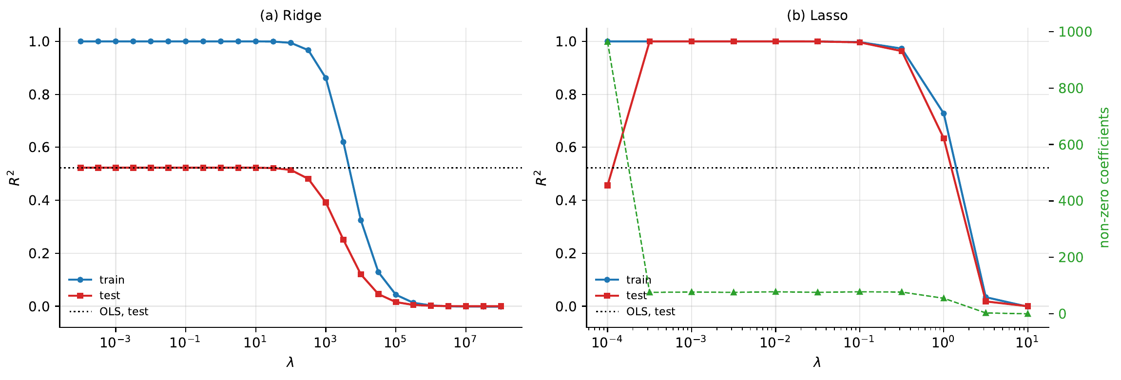
Figure 3.10: Test and training \(R^{2}\) against the penalty for the Ising problem, with the OLS test score marked. Ridge (a) needs \(\lambda\sim10^{3}\) before anything happens, and never beats OLS. The Lasso (b) has a broad plateau on which it is exact, and the count of non-zero coefficients (right axis, dashed) sits at about \(2L=80\) across it.
3.16.5. What the example is for#
The headline is that on a problem with a sparse truth the Lasso reached \(R^{2}=0.99996\) on unseen data from \(400\) samples and \(1600\) parameters, while OLS and Ridge reached \(0.52\). But the headline is the least transferable part, because it is a consequence of the truth being sparse in the basis we chose, and we chose the basis knowing the answer. Three things generalise.
First, the failure of OLS and Ridge is not a failure of computation. Both returned the correct minimiser of the objective they were given; the objective was simply the wrong one, because \(819\) directions in parameter space leave the training energies unchanged and something other than the data must decide what happens along them. Ridge decides by the \(2\)-norm and the Lasso by the \(1\)-norm, and Proposition 3.15 says exactly what each choice does. This is the content of Section A Bayesian reading made concrete: in the underdetermined regime the penalty is the model.
Second, sparsity and symmetry are in conflict, and one has to choose. The Lasso got the physics right in the only sense the data allow – the sum \(J_{jk}+J_{kj}\) – and got the presentation wrong, reporting a coupling matrix that is not symmetric although the underlying interaction certainly is. If a symmetric answer is wanted, the honest fix is not to post-process the Lasso but to remove the redundancy from the design matrix beforehand, keeping one column per unordered pair \(j<k\) and none of the diagonal. That reduces \(p\) from \(1600\) to \(781\), makes the design matrix full rank by Proposition 3.14, and is what one should do in practice. We kept the redundant parametrisation here precisely because the pathology it produces is instructive.
Third, and most important for what follows: everything above depended on someone knowing to build the features \(s_js_k\). The linear model never saw a spin, only a product of two spins, and the products were supplied by a physicist who already suspected a pairwise interaction. Section An extended example: learning the Ising energy returns to this same chain with a neural network, hands it the raw spins with no products at all, and asks whether the features can be discovered rather than assumed. The answer involves a theorem, and a caution.
Machine learning connection
Discovering an interaction from configurations and energies is a real and active use of regression in statistical physics and in materials science, where it is called inverse statistical mechanics or, in the lattice-model community, cluster expansion: one fits an effective Hamiltonian to energies computed by an expensive first-principles method, and then uses the fitted model in place of the expensive one. Everything this section illustrates matters there. The candidate interactions vastly outnumber the configurations one can afford to compute, the physically correct answer is sparse – few clusters contribute appreciably – and symmetry makes whole groups of features exactly exchangeable. Practitioners consequently reach for the Lasso and for structured variants of it, and they take care to remove symmetry-equivalent duplicates from the design matrix before fitting rather than after, for the reason Proposition 3.15 gives.
3.17. Summary and the programs#
Linear regression has given us, in closed form, every quantity the rest of this book will only be able to estimate.
The estimator itself arrived three times over. As an optimisation problem it is the minimiser of the squared error, Eq. (3.8); as geometry it is the orthogonal projection of the targets onto the column space of the design matrix, Eq. (3.9); and as statistics it is the maximum-likelihood estimate under Gaussian noise, Eq. (3.28). The three derivations are worth holding together, because each generalises differently: the first survives into every method in this book, the second is what makes the linear case special, and the third is what tells us that a different noise model demands a different loss.
The statistics of the estimator all flow from one object, the residual projector \(\bm{I}-\bm{H}\), which annihilates the model and leaves the noise: it gives the divisor \(n-p\) in \(\hat{\sigma}^{2}\), the \(\chi^{2}_{n-p}\) distribution behind the reduced \(\chi^{2}\) and the \(t\) intervals, the optimism \(2p\sigma^{2}/n\) of the training error, and through its diagonal the leave-one-out formula (3.39).
The three penalties then formed a sequence. Ordinary least squares is unbiased and, by Gauss-Markov (Theorem 3.4), of minimum variance among unbiased linear estimators – and that guarantee is worth less than it sounds, because Eq. (2.27) counts variance alongside bias. Ridge regression buys a large reduction in variance for a small bias, shrinking each singular direction by \(\sigma_i^{2}/(\sigma_i^{2}+\lambda)\) and hence suppressing hardest exactly those directions in which Eq. (3.42) shows the data to be least informative. The Lasso replaces proportional shrinkage by soft thresholding (3.63), and thereby sets coefficients exactly to zero – a difference which is visible in the algebra, in the geometry of the \(1\)-norm ball, and in the shape of the corresponding Laplace prior.
The Bayesian reading of Section A Bayesian reading unified the three: a flat prior gives OLS, a Gaussian prior gives Ridge, a Laplace prior gives the Lasso. Regularisation is the expression of a prior belief, and the regularisation parameter is its strength.
Finally, none of this survives careless practice. Penalties are meaningless unless the features are on comparable scales; the intercept must be excluded from the penalty; every transformation must be fitted on training data alone; and the number one reports must come from data the model has never seen. The penalty itself is chosen by the cross-validation of Section Choosing the penalty: cross-validation for Ridge and Lasso: a logarithmic grid, \(K\) folds with the standardisation inside each, the minimum of Eq. (3.92) or the one-standard-error choice (3.96), a refit on all training data, and one look at the test set. Cross-validation is preferred to the bootstrap for this purpose because its bias is nearly constant in \(\lambda\) and so leaves the minimum in place, because it costs \(K\) fits rather than hundreds, and because its models see \((K-1)/K\) of the data rather than the \(63\%\) of Eq. (3.97); the bootstrap keeps its role of estimating the distribution of whatever cross-validation selects, above all the Lasso’s support.
A last thread runs underneath all three estimators and is the subject of Section Kernel methods: regression without coordinates. The \(2\)-norm penalty is invariant under a change of orthonormal basis in the feature space, so it can be expressed through inner products alone; the push-through identity of Lemma 3.10 then rewrites Ridge regression in terms of the \(n\times n\) matrix of those inner products, the basis expansion becomes free, and Theorem 3.12 shows that the same is true for any loss. The \(1\)-norm is not invariant, Proposition 3.13, and the Lasso therefore does not kernelise – which is worth knowing, because the literature contains two different repairs travelling under the same name.
The complete programs are collected in doc/BookML/BookPrograms:
kernel_regression.py– the push-through identity, the Hoerl-Kennard theorem, kernel ridge regression againstscikit-learnand against an explicit feature map, the rotation counter-example of Proposition 3.13, and both repairs of Section There is no kernel Lasso.linear_regression.py– OLS by the SVD, by QR and by the normal equations, with the conditioning comparison of Section Ordinary least squares; weighted least squares and the reduced-\(\chi^{2}\) simulation of Section Weighted least squares and the \(\chi^2\) function; the quality measures of Section Measures of quality; and the checks of Section Statistical properties of the least-squares estimator – unbiasedness of \(\hat{\sigma}^{2}\), coverage of the \(t\) intervals, the optimism formula (3.37) and leave-one-out in closed form.ridge_lasso.py– Ridge in closed form and through the SVD, the Lasso by coordinate descent with soft thresholding, and the coefficient paths of Section Comparing the three estimators compared against the analytical results.cross_validation.py– the procedure of Section Choosing the penalty: cross-validation for Ridge and Lasso from scratch: \(K\)-fold cross-validation with standardisation inside the folds for Ridge and the Lasso, the minimum-CV and one-standard-error choices, the refit and the single test evaluation, theGridSearchCVequivalent checked to rounding error, the leave-one-out bootstrap and .632 estimators against cross-validation and the true error, the repeated experiment behind the bias and spread table, and the bootstrap selection frequencies of the Lasso support.franke.py– the complete study of Section A complete example: the Franke function: design matrices for two-dimensional polynomials, the train-test split, cross-validated selection of \(\lambda\), test error against polynomial degree for all three methods, and the count of non-zero Lasso coefficients.scaling.py– the intercept and standardisation conventions of Section Scaling, centring and the intercept, with a reconciliation of a hand-written implementation againstscikit-learn.ising_regression.py– the one-dimensional Ising study of Section A second example: the one-dimensional Ising model: the exact rank deficiency of Proposition 3.14, the three estimators at \(p=4n\), the duplicated-column symmetry of Proposition 3.15 and the indifference of the Lasso objective to the split, and the penalty scan over eight decades.
Each file runs as a script and reproduces the numbers quoted in this chapter. An executable version is available as a Jupyter notebook in the accompanying Jupyter-book.
3.18. Exercises#
3.18.1. Warm-up exercises#
The normal equations by hand. For the toy problem of Eq. (3.70): (a) compute \(\bm{X}^{T}\bm{X}\) and \(\bm{X}^{T}\bm{y}\) and verify Eq. (3.72); (b) compute the hat matrix (3.9) and verify that it is symmetric, idempotent, and has trace \(2\); (c) verify that the residual is orthogonal to both columns of \(\bm{X}\).
Ridge by hand. For the same problem, derive Eq. (3.73) by differentiating the penalised cost, and explain why the two coefficients are shrunk by different factors. Relate the factors to the singular values of \(\bm{X}\).
The Lasso threshold. For the same problem, show that the Lasso sets \(\theta_1=0\) for \(\lambda\ge4\) and \(\theta_0=0\) for \(\lambda\ge16\) (with the convention of Eq. (3.57) and the \(1/n\) dropped). Sketch all three coefficient paths on one plot.
Equivariance under rescaling. (a) Show that if a column of \(\bm{X}\) is multiplied by \(c\), the OLS fitted values \(\tilde{\bm{y}}\) are unchanged while the corresponding coefficient is divided by \(c\). (b) Show that this fails for Ridge, and explain in one sentence why standardisation is therefore mandatory for penalised regression and optional for OLS.
Maximum likelihood with a different noise model. Repeat the derivation of Section Deriving least squares from a probability distribution assuming Laplace noise, \(p(\varepsilon)\propto\exp(-|\varepsilon|/b)\). Which cost function results? What does this say about the robustness of the two fits to outliers?
Degrees of freedom. (a) Show that \(\mathrm{Tr}(\bm{H})=p\) for the OLS hat matrix. (b) Show that the Ridge analogue \(\bm{H}_\lambda=\bm{X}(\bm{X}^{T}\bm{X}+\lambda\bm{I})^{-1}\bm{X}^{T}\) has trace \(\sum_i\sigma_i^{2}/(\sigma_i^{2}+\lambda)\), which is Eq. (1.132). (c) Verify that \(\bm{H}_\lambda\) is symmetric but not idempotent for \(\lambda>0\), and interpret this using the eigenvalue argument of Section Orthonormal bases and projections.
The analysis-of-variance identity. (a) Show that if the design matrix has no constant column, the residuals of a least-squares fit need not sum to zero, and give a two-point example in which Eq. (3.20) fails. (b) Show that for a fit with intercept the sample correlation between \(\bm{y}\) and \(\tilde{\bm{y}}\) squared equals \(R^{2}\). (c) Compute \(R^{2}\) and \(\bar{R}^{2}\) of Eq. (3.22) for a polynomial fit of degree \(1,\dots,15\) to \(20\) noisy points and plot both against the degree.
Generalised least squares. Noise with an autoregressive structure has covariance \(\Omega_{ij}=\sigma^{2}\rho^{|i-j|}\). (a) Simulate such noise for \(\rho=0.8\) and fit a straight line by OLS and by GLS, Eq. (3.15), many times; compare the empirical variances of the slope with the two predicted covariance matrices. (b) Show that the OLS variance formula \(\sigma^{2}(\bm{X}^{T}\bm{X})^{-1}\) is wrong in this case, and derive the correct \(\var(\hat{\bm{\theta}}_{\mathrm{OLS}}) =(\bm{X}^{T}\bm{X})^{-1}\bm{X}^{T}\bm{\Omega}\bm{X}(\bm{X}^{T}\bm{X})^{-1}\).
The Cram’er-Rao bound for the noise variance. Compute the Fisher information for \(\sigma^{2}\) from Eq. (3.27), \(\mathcal{I}(\sigma^{2})=n/(2\sigma^{4})\), and hence the bound \(\var(\tilde{\sigma}^{2})\ge2\sigma^{4}/n\). Using Proposition 3.3(iii), show that \(\var(\hat{\sigma}^{2})=2\sigma^{4}/(n-p)\): the unbiased estimator does not attain the bound, and the gap closes as \(p/n\to0\).
Leave-one-out by Sherman-Morrison. (a) Verify Eq. (3.38) by multiplication. (b) Derive both parts of Eq. (3.39); the key step is \(\bm{x}_i^{T}(\bm{X}^{T}\bm{X})^{-1}\bm{x}_i=h_{ii}\). (c) Show that \(0\le h_{ii}\le1\) and \(\sum_ih_{ii}=p\), so that the average leverage is \(p/n\); explain what happens to Eq. (3.39) at a point with \(h_{ii}=1\). (d) Repeat the numerical comparison of Section Statistical properties of the least-squares estimator for the Ridge smoother, and confirm that Eq. (3.40) still holds with \(S_{ii}\) in place of \(h_{ii}\).
Optimism (numerical). For polynomial fits of degree \(d=1,\dots,12\) to \(n=30\) points generated by a cubic plus Gaussian noise, estimate by simulation the expected training and test errors and plot both against \(d\) together with the predictions (3.35) and (3.36). Where do the predictions fail, and why? Add Mallows’ \(C_p\) and check that its minimum sits at the true degree.
Conditioning in practice (numerical). Fit a polynomial of degree \(d\) to \(100\) points on \([0,1]\) using both functions of Section Ordinary least squares. (a) For \(d=2,4,\dots,14\), compare the coefficients returned by the two. (b) Plot \(\kappa_2(\bm{X})\) and \(\kappa_2(\bm{X}^{T}\bm{X})\) against \(d\). (c) At which \(d\) do the two methods first disagree in the first significant digit, and how does that relate to Eq. (1.118)?
Coordinate descent (numerical). Implement the Lasso by coordinate descent as in Eq. (3.69). (a) Verify on an orthonormal design that it reproduces the soft thresholding result (3.63) exactly. (b) Compare against
sklearn.linear_model.Lassoon a general design, taking care over the factor conventions noted in Section Comparing the three estimators. (c) Plot the number of non-zero coefficients against \(\lambda\).Confidence intervals (numerical). For data generated from a known linear model: (a) compute the confidence intervals (3.34) for each coefficient; (b) repeat the whole experiment \(1000\) times with fresh noise and count how often the true value lies inside the interval; (c) does the coverage match the nominal \(95\%\)? Repeat with two nearly collinear columns and comment.
Ridge and the bias-variance trade-off (numerical). For a fixed polynomial degree, plot the squared bias, the variance and the test error of a Ridge fit against \(\lambda\), using the bootstrap procedure of Section The bias-variance tradeoff. Verify that the bias increases monotonically, the variance decreases monotonically, and the minimum of the sum occurs at \(\lambda>0\).
The training error is monotone in the penalty. Let \(\hat{\bm{\theta}}(\lambda)\) minimise \(L(\bm{\theta})+\lambda P(\bm{\theta})\) for a loss \(L\) and a penalty \(P\), both arbitrary. For \(\lambda_1<\lambda_2\) write down the two inequalities expressing that each minimiser beats the other at its own penalty, add them, and conclude that \(P(\hat{\bm{\theta}}(\lambda_2))\le P(\hat{\bm{\theta}}(\lambda_1))\) and \(L(\hat{\bm{\theta}}(\lambda_1))\le L(\hat{\bm{\theta}}(\lambda_2))\). This proves Eq. (3.91) along the whole path, for Ridge and the Lasso alike, and shows that the training error can never select a penalty. Verify it numerically on the dotted curves of Figure 3.4.
The factor \(n\). (a) Show that the minimiser of \(\|\bm{y}-\bm{X}\bm{\theta}\|_2^{2}/n +\lambda\|\bm{\theta}\|_2^{2}\) is Eq. (3.95), and that the same estimator minimises \(\|\bm{y}-\bm{X}\bm{\theta}\|_2^{2} +\lambda'\|\bm{\theta}\|_2^{2}\) with \(\lambda'=n\lambda\). (b) A penalty \(\lambda'\) is selected by five-fold cross-validation in the second convention and then used to refit on all \(n\) training points. By what factor is the effective per-observation penalty changed between selection and refit, and in which direction? (c) Repeat the
GridSearchCVrun of Section Choosing the penalty: cross-validation for Ridge and Lasso withalphaset to \(100\lambda\) instead of \(80\lambda\) and confirm the shift of one grid point.Out of the bag. (a) Prove Eq. (3.97) and evaluate \((1-1/n)^{n}\) for \(n=10\), \(100\) and \(1000\). (b) Show that the expected number of distinct observations in a bootstrap sample is \(n[1-(1-1/n)^{n}]\), and that the expected number of replicas out of \(B\) in which a given observation is absent is \(B(1-1/n)^{n}\); hence explain why the
seenmask in the code of Section Choosing the penalty: cross-validation for Ridge and Lasso is almost never needed for \(B=200\). (c) For which \(K\) does \(K\)-fold cross-validation train on the same fraction of the data as the leave-one-out bootstrap?The one-standard-error rule (numerical). For the sparse problem of Section Choosing the penalty: cross-validation for Ridge and Lasso, generate \(200\) training sets and, for each, select the Lasso penalty by the minimum-CV rule and by the one-standard-error rule. (a) Record for each rule the number of retained coefficients, the number of true coefficients retained, and the true test error measured on a large fresh sample. Report the averages. (b) Which rule retains fewer spurious coefficients, and what does it cost in test error on average? (c) Repeat with \(\rho=0\) and with \(\rho=0.9\) and explain what the correlation between features does to both rules.
Nested cross-validation (numerical). Without using a test set, estimate the generalisation error of the complete Ridge procedure of Section Choosing the penalty: cross-validation for Ridge and Lasso – grid, five-fold selection, refit – by nesting it in an outer five-fold loop. Compare the outer estimate with \(\mathrm{CV}_5(\lambda_{\min})\) from the inner loop and with the true error from a large fresh sample, then repeat with a grid of \(600\) penalties instead of \(60\) and with \(n=40\) instead of \(100\). When does the difference between the inner minimum and the outer estimate become important?
3.18.2. Project-style exercise: regression analysis of the Franke function#
This extended exercise assembles the whole chapter, and follows the structure of the first project of the course.
Part a: ordinary least squares. Generate a data set from the Franke function (3.100) with \(x,y\in[0,1]\) and added noise \(\mathcal{N}(0,\sigma^{2})\). Write your own code – using either a matrix inversion or, preferably, the singular value decomposition – and perform a standard least-squares analysis with polynomials in \(x\) and \(y\) up to fifth order.
Part b: the bias-variance trade-off with the bootstrap. Using the bootstrap of Section Resampling: the jackknife and the bootstrap, decompose the test error into bias and variance as in Eq. (2.52) and plot all three against polynomial degree. Explain the shape of each curve. Then repeat with a substantially larger data set and account for the shift in the optimum.
Part c: cross-validation. Implement \(k\)-fold cross-validation from scratch, with \(k\) between five and ten, and compare its estimate of the test error with the bootstrap estimate of part b. Which is cheaper, and which has the smaller variance? Relate your findings to the comparison of Section Choosing the penalty: cross-validation for Ridge and Lasso, in particular to the fraction of distinct observations in a bootstrap sample, Eq. (3.97).
Part d: Ridge regression. Repeat parts a to c for Ridge regression, as a function of both the polynomial degree and the penalty \(\lambda\). Present your results as a heat map of the cross-validated test error over the two hyperparameters, and identify the optimum. Discuss the results in the light of the shrinkage (3.48) and of the variance difference (3.52).
Part e: the Lasso.
Repeat part d for the Lasso, using either your own coordinate-descent
implementation or scikit-learn. In addition, count the non-zero
coefficients at the optimal \(\lambda\) and compare with the number retained by
Ridge. Which monomials survive, and does the selection agree with your
expectation from the shape of the Franke surface?
Part f: real data. Finally, replace the Franke function by a real data set – digital terrain data are a natural choice, being a genuine two-dimensional surface – and repeat the analysis. Discuss what changes when the true function is unknown, the noise level is unknown, and the observations may be spatially correlated. In particular, reconsider whether a random train-test split is defensible, in the light of Section Correlated data and the autocorrelation function.