
17. Chapter 17: Generative Adversarial Networks#
Every generative model of Chapters 14 to 16 was built around the likelihood. The restricted Boltzmann machine of Chapter 14 wrote down an unnormalised density and struggled with the partition function; the variational autoencoder of Chapter 15 replaced the intractable \(\log p(\bm{x})\) by a bound; the diffusion model of Chapter 16 replaced it by a bound with \(T\) terms. In each case the object being optimised was, directly or indirectly, the probability the model assigns to the data.
This chapter is about giving that up. A generative adversarial network never evaluates \(p_{\bm{\theta}}(\bm{x})\), never bounds it, and never approximates a partition function. It trains a generator by asking a second network – a discriminator – whether the generated samples look real, and improves the generator until the discriminator can no longer tell. The training signal is not a likelihood but the output of a classifier that is being retrained at the same time.
The construction is due to Goodfellow and coworkers [goodfellow2014gan] and it is best read as a two-player game. That reading is what gives the chapter its structure: we shall write down the value function of the game (Section The minimax objective), solve it for one player exactly (Section The optimal discriminator), show that the resulting objective for the other player is a Jensen-Shannon divergence (Section The objective is a Jensen-Shannon divergence), and then spend the rest of the chapter on the consequences – both the good ones, which are the sharpest samples any single-pass generator produces, and the bad ones, which are that the game may fail to converge at all.
The material follows the lecture notes for the last week of FYS-STK4155 and the accompanying notes on generative adversarial networks; Chapter 20 of Goodfellow, Bengio and Courville [goodfellow2016] is the standard textbook treatment. Every identity stated below is verified numerically by the programs described in Section Summary and the programs: no result in this chapter is quoted without having been recomputed.
17.1. Two networks and a game#
A generative adversarial network consists of two networks with opposing objectives.
The generator \(G\) takes a noise vector \(\bm{z}\in\mathbb{R}^{k}\) drawn from a fixed prior \(p_{z}\) – usually \(\mathcal{N}(\bm{0},\bm{I})\) or a uniform distribution on a cube – and maps it into data space,
The distribution of the output is written \(p_{g}\). It is the push-forward of \(p_z\) through \(G\), and this is the first thing that distinguishes a GAN from everything that came before: we can sample from \(p_g\) by drawing \(\bm{z}\) and applying one forward pass, but we cannot in general evaluate it. If \(G\) happened to be a diffeomorphism the change of variables of Chapter 16, Theorem 16.5, would give
but \(G\) is a generic network with \(k\ne d\) and no invertibility constraint, so Eq. (17.2) does not apply. We call \(p_g\) an implicit distribution: defined by a sampling procedure and nothing else.
The discriminator \(D\) takes a point in data space and returns a probability,
which we shall always implement as a sigmoid applied to a real-valued logit \(u(\bm{x})\), so that \(D=\sigma(u)\) and the losses below can be written with the softplus function and evaluated without overflow.
The two are trained against each other. The generator wants \(D(G(\bm{z}))\) large; the discriminator wants \(D(\bm{x})\) large on data and \(D(G(\bm{z}))\) small on samples. Neither network ever sees the other’s parameters: all the information the generator receives about the data arrives through the discriminator’s gradient.
Supervised, unsupervised, or neither?
A GAN is normally listed as an unsupervised method, and the end product – a model of \(p_r\) built from unlabelled samples – justifies that. But internally the discriminator solves a perfectly ordinary supervised binary classification problem, with labels that the construction supplies for free: real is \(1\), generated is \(0\). The unsupervised task has been converted into a supervised one, at the price that the training set for the classifier changes at every step. This is why GANs extend so naturally to the semi-supervised setting, where the discriminator is given \(C+1\) classes – the \(C\) real classes plus “generated” – and the unlabelled data still contribute through the adversarial term.
17.1.1. What GANs are used for#
The applications that made GANs prominent are almost all in image space: synthesis of photorealistic faces and scenes, super-resolution, inpainting, image-to-image translation between paired or unpaired domains, style transfer, text-to-image generation, video prediction and face ageing. In the physical sciences they have been used for fast surrogate simulation – generating calorimeter showers or lattice configurations far more cheaply than the underlying simulator – for data augmentation when the interesting events are rare, and for anomaly detection through the reconstruction error of an inverted generator.
What all of these share is that the target is a sharp, high-dimensional signal for which no tractable likelihood is available and for which a pixel-wise loss is known to be the wrong criterion. That is the regime where an adversarial loss earns its cost, and Section What actually goes wrong is about what that cost is.
17.2. The minimax objective#
The learning problem is posed as a zero-sum game. A single function \(V(G,D)\) gives the reward of the discriminator; the generator receives \(-V\). The default choice is
Read the two terms separately. The first is large when \(D\) assigns high probability to real data. The second is large when \(D\) assigns low probability to generated data. Maximising their sum over \(\bm{\theta}^{(d)}\) is exactly maximum likelihood for a binary classifier with balanced classes – the right-hand side of Eq. (17.4) is the negative binary cross-entropy of Chapter 5, Eq. (5.13), with the two classes “real” and “generated”.
Since \(G\) appears only in the second term, minimising \(V\) over \(\bm{\theta}^{(g)}\) means minimising \(\mathbb{E}_{\bm{z}}[\log(1-D(G(\bm{z})))]\); the generator is pushing \(D(G(\bm{z}))\) up. Changing variables from \(\bm{z}\) to \(\bm{x}=G(\bm{z})\) lets us write the same thing entirely in data space,
which is the form we shall analyse. Note what has happened: the parameters \(\bm{\theta}^{(g)}\) have disappeared into \(p_g\), and the game is now a game between two distributions, \(p_g\) and \(D\). Everything in the next two sections is a statement about that idealised game; Section Training: alternating gradients returns to the parameters.
In the numerical work we write the two terms with the softplus function \(\zeta(u)=\log(1+e^{u})\), using \(\log\sigma(u)=-\zeta(-u)\) and \(\log(1-\sigma(u))=-\zeta(u)\):
def softplus(u):
    """log(1+exp(u)), evaluated without overflow."""
    return np.maximum(u, 0.0) + np.log1p(np.exp(-np.abs(u)))


def value_function(Q, P, x_real, z):
    """V(G,D) = E[log D(x)] + E[log(1 - D(G(z)))],  Eq. (17.minimax)."""
    u_real = discriminator(Q, x_real)
    u_fake = discriminator(Q, generator(P, z))
    return -np.mean(softplus(-u_real)) - np.mean(softplus(u_fake))
17.3. The optimal discriminator#
Hold the generator fixed, so that \(p_g\) is a fixed distribution, and ask for the discriminator that maximises Eq. (17.5). Because \(D\) enters the integral pointwise – the value of \(D\) at one \(\bm{x}\) does not constrain its value at another, if we optimise over all measurable functions – the problem separates into one scalar maximisation per point.
Proposition 17.1 (Optimal discriminator)
For fixed \(p_g\), the value function Eq. (17.5) is maximised by
at every \(\bm{x}\) with \(p_r(\bm{x})+p_g(\bm{x})>0\).
Proof
Write \(A=p_r(\bm{x})\), \(B=p_g(\bm{x})\) and \(t=D(\bm{x})\in(0,1)\). The integrand is \(f(t)=A\log t + B\log(1-t)\), and
which vanishes at \(t^{*}=A/(A+B)\). The second derivative,
is negative wherever \(A\) and \(B\) are not both zero, so \(f\) is strictly concave and \(t^{*}\) is its unique maximum. Since the choice of \(t\) at one point does not affect any other point, maximising the integrand pointwise maximises the integral.
Equation (17.6) is worth reading twice. It says the optimal discriminator is the Bayes-optimal classifier for the two-class problem \(\{\)real, generated\(\}\) with equal class priors: the posterior probability that a point came from \(p_r\) rather than \(p_g\). A perfectly trained discriminator is therefore not an adversary in any mysterious sense; it is a density ratio estimator. Rearranging,
so the logit of the optimal discriminator is the log density ratio. The generator is being told, at every point, how much too little or too much mass it has put there – which is precisely the information a likelihood would have given, obtained without ever computing one.
We check Proposition 17.1 in two ways. First, pointwise: for several pairs \((A,B)\) we maximise \(f(t)\) numerically and compare against \(A/(A+B)\),
=== 1. the pointwise maximiser of A log t + B log(1-t) ===
      A          B        numerical t*       A/(A+B)      |diff|
    0.9000     0.1000     0.9000000001  0.9000000000   1.1e-10
    0.5000     0.5000     0.5000000000  0.5000000000   1.1e-16
    0.2000     0.8000     0.1999999970  0.2000000000   3.0e-09
    0.0010     0.4000     0.0024937656  0.0024937656   3.5e-11
    0.3700     0.1100     0.7708333325  0.7708333333   8.7e-10
  worst deviation from Eq. (17.dstar): 2.97e-09

  f''(t*) = -2.7172 < 0, so t* is a maximum
Second, and more interestingly, with a network. We take two known one-dimensional densities, \(p_r=\mathcal{N}(0,1)\) and \(p_g=\mathcal{N}(1.5,0.6^{2})\), draw twenty thousand samples from each, and train a discriminator on the binary cross-entropy of Eq. (17.4) with the generator frozen. Nothing in the training knows the densities; the network sees only samples. Comparing the trained \(D\) against Eq. (17.6):
=== 2. a trained discriminator against a known pair of densities ===
     x        mixture     D_net(x)   p_r/(p_r+p_g)   |diff|
   -2.00     2.70e-02    0.99998        1.00000    0.0000
    0.00     2.14e-01    0.91331        0.93177    0.0185
    1.00     3.56e-01    0.38890        0.33993    0.0490
    2.00     2.62e-01    0.13343        0.10307    0.0304
    3.00     1.68e-02    0.11105        0.13172    0.0207
    4.00     1.23e-04    0.09246        0.54233    0.4499
    5.00     7.57e-07    0.07672        0.98207    0.9053
  where the mixture density exceeds 1% of its peak (x in [-2.77,3.33]):
      max |D_net - D*| = 0.0911, rms = 0.0240
  over the whole grid, including the empty tails:
      max |D_net - D*| = 0.9053, rms = 0.2647
  V from the trained network : -0.753844
  2 JS - 2 log 2 by quadrature: -0.751959
Two things should be noticed. Where there are data the network reproduces Eq. (17.6) to a root-mean-square error of \(0.024\), which is what one expects from twenty thousand samples and a network of this size. Where there are no data – at \(x=5\) the mixture density is \(7.6\times10^{-7}\) – it is wrong by \(0.9\), and confidently so. Figure 17.1 shows this. It is the first hint of a theme that runs through the whole chapter: statements about \(D^{*}\) are statements about the region where \(p_r+p_g\) is appreciable, and the generator receives no reliable guidance anywhere else. The last two lines of the output anticipate the next section.
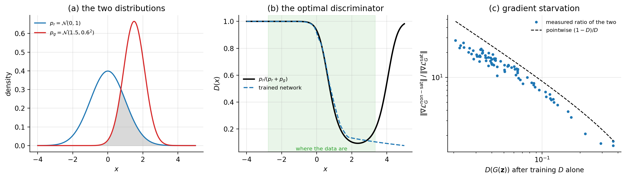
Figure 17.1: (a) The two one-dimensional distributions used to test Proposition 17.1, with their overlap shaded. (b) The trained discriminator against the closed form \(p_r/(p_r+p_g)\) of Eq. (17.6); the shaded band marks where the mixture density exceeds one per cent of its peak. Inside it the agreement is \(0.024\) rms; outside it the network is arbitrary, because no sample ever landed there. (c) The ratio of the two generator gradients of Section The non-saturating generator loss, measured while training the discriminator alone against a frozen generator, against the pointwise prediction \((1-D)/D\) of Eq. (17.19).
17.4. The objective is a Jensen-Shannon divergence#
We now substitute Eq. (17.6) back into the value function and ask what the generator is really minimising. Two divergences are needed.
The Kullback-Leibler divergence of Chapter 14, Section The same statement as a divergence, is
with equality if and only if \(p=q\) almost everywhere. It is not symmetric and it is infinite whenever \(p\) puts mass where \(q\) puts none.
The Jensen-Shannon divergence repairs both defects by comparing each distribution to their mixture \(m=\tfrac{1}{2}(p+q)\):
Lemma 17.2 (Range of the Jensen-Shannon divergence)
\(0\le D_{\mathrm{JS}}(p\|q)\le\log 2\) for any pair of distributions, with \(D_{\mathrm{JS}}=0\) if and only if \(p=q\) almost everywhere and \(D_{\mathrm{JS}}=\log 2\) if and only if \(p\) and \(q\) have disjoint supports.
Proof
Non-negativity and the equality case follow from those of \(D_{\mathrm{KL}}\), since \(m=p\) almost everywhere forces \(p=q\). For the upper bound write out Eq. (17.11),
and note that \(p/(p+q)\le1\) and \(q/(p+q)\le1\) pointwise, so both integrals are \(\le0\) and \(D_{\mathrm{JS}}\le\log2\). Equality requires \(p\log\bigl(p/(p+q)\bigr)=0\) and \(q\log\bigl(q/(p+q)\bigr)=0\) almost everywhere, that is, \(q=0\) wherever \(p>0\) and conversely: disjoint supports.
The bound \(\log2\) is the whole story of Section The Wasserstein distance, so it is worth having proved rather than quoted.
Theorem 17.3 (The value at the optimum)
With \(D^{*}\) of Eq. (17.6),
Consequently \(V(G,D^{*})\ge-2\log2\), with equality if and only if \(p_g=p_r\), and at that point \(D^{*}\equiv\tfrac{1}{2}\).
Proof
Substituting Eq. (17.6) into Eq. (17.5),
where in the second line we multiplied and divided each argument of the logarithm by \(2\), each such step contributing \(-\log2\) because \(p_r\) and \(p_g\) integrate to one. The bracket is Eq. (17.11). The bound then follows from Lemma 17.2, and \(p_g=p_r\) gives \(D^{*}=p_r/(2p_r)=\tfrac{1}{2}\) directly from Eq. (17.6).
So the game, played to the discriminator’s optimum at every step, is
a statement of remarkable economy: fitting a classifier and then fooling it is the same thing as minimising a symmetric divergence between the model and the data. The value \(-2\log2\approx-1.386\) is the signature of success, and \(D\equiv\tfrac{1}{2}\) is the signature the practitioner actually monitors, since \(V\) requires \(D^{*}\) and \(D\) is available directly.
Both statements are checked by quadrature on one-dimensional Gaussians, where the JS divergence can be computed independently:
=== 3. the value at the optimal discriminator is the JS divergence ===
   m_g   s_g      V(G,D*)       2 JS - 2log2        |diff|      JS
   0.0   1.0   -1.38629436     -1.38629436    2.24e-12   0.00000
   0.5   1.0   -1.32567176     -1.32567176    2.24e-12   0.03031
   1.5   0.6   -0.75195864     -0.75195864    2.24e-12   0.31717
   3.0   1.0   -0.33273975     -0.33273975    1.35e-12   0.52678
   6.0   0.8   -0.00249849     -0.00249869    1.99e-07   0.69190
  the equal case p_g = p_r gives V = -2log2 = -1.38629436 and D* = 1/2
  the JS divergence is bounded by log 2 = 0.69314718
The agreement is at the level of the quadrature, \(10^{-12}\). The last row is the case that Section The Wasserstein distance is about: two Gaussians six standard deviations apart have \(D_{\mathrm{JS}}=0.6919\), within \(10^{-3}\) of the ceiling \(\log2=0.6931\), and \(V(G,D^{*})\) has correspondingly flattened to \(-0.0025\). Moving them further apart changes almost nothing.
Which divergence, and why it matters
The VAE of Chapter 15 minimises \(D_{\mathrm{KL}}(q\|p)\) in the latent space and maximises a likelihood in data space, which amounts to minimising the forward divergence \(D_{\mathrm{KL}}(p_r\|p_g)\). That divergence is infinite wherever the model assigns zero density to real data, so it is mode-covering: the model is heavily punished for missing anything and will spread mass over regions with no data rather than risk a gap. Blur is the visible symptom.
The reverse divergence \(D_{\mathrm{KL}}(p_g\|p_r)\) punishes putting mass where there are no data but not the converse, and is therefore mode-seeking: it is content to model one mode well and ignore the rest. The Jensen-Shannon divergence of Eq. (17.11) is a symmetrised average of the two and sits between them – which is why GAN samples are sharper than VAE samples and why GANs, unlike VAEs, can quietly drop modes. Sharpness and mode dropping are two readings of the same choice of divergence, not two independent facts.
17.5. Training: alternating gradients#
The theory of the previous two sections assumed that \(D\) reaches its optimum for each \(G\). In practice we can afford neither an inner optimisation to convergence nor an optimisation over all measurable functions, and we take one gradient step for each player in turn. One iteration is
Freeze \(\bm{\theta}^{(g)}\) and take \(n_{\mathrm{critic}}\) ascent steps on the discriminator,
\[ \bm{\theta}^{(d)} \leftarrow \bm{\theta}^{(d)} + \gamma_d\,\nabla_{\bm{\theta}^{(d)}}V(G,D),\tag{17.15} \]where \(V\) is estimated on a minibatch of real data and a minibatch of generated data. The generated batch is detached from the computational graph, so that no gradient reaches \(\bm{\theta}^{(g)}\) here.
Freeze \(\bm{\theta}^{(d)}\) and take one descent step on the generator,
\[ \bm{\theta}^{(g)} \leftarrow \bm{\theta}^{(g)} - \gamma_g\,\nabla_{\bm{\theta}^{(g)}}\mathcal{L}_G .\tag{17.16} \]
The usual choice is \(n_{\mathrm{critic}}=1\): the discriminator is kept near its optimum rather than at it, and the theory of Section The objective is a Jensen-Shannon divergence is an idealisation of what the algorithm does. In terms of minibatch estimates the two losses are
which is \(-V\) estimated on the batch, and the generator loss of the next subsection.
17.5.1. The non-saturating generator loss#
Equation (17.4) says the generator should minimise \(\mathbb{E}[\log(1-D(G(\bm{z})))]\). This is a bad idea, and the reason is worth deriving rather than asserting.
Write \(u=u(G(\bm{z}))\) for the discriminator logit at a generated point, so that \(D=\sigma(u)\). Then
Both losses reach \(\bm{\theta}^{(g)}\) through the same chain \(\partial u/\partial\bm{\theta}^{(g)}\), so the two gradients differ only by the scalar prefactor, and their ratio is
pointwise. Early in training the discriminator wins easily and \(D(G(\bm{z}))=\varepsilon\ll1\). The saturating gradient is then proportional to \(\varepsilon\) and vanishes; the non-saturating one is proportional to \(1-\varepsilon\approx1\) and does not. The generator is starved of gradient exactly when it is worst and most needs one. The remedy, which is what everyone uses, is to replace minimising \(\log(1-D)\) with maximising \(\log D\):
Both losses are minimised by the same \(G\) – both are decreasing functions of \(D(G(\bm{z}))\) – so the fixed point of the game is unchanged. Only the gradient magnitudes differ, and Eq. (17.19) says by how much. Note that Eq. (17.20) is no longer the negative of anything the discriminator maximises: the game is no longer zero-sum, only adversarial.
The prefactors of Eq. (17.18) are confirmed by automatic differentiation:
=== 5. the two generator losses at D(G(z)) = eps ===
      eps     |dL_sat/du|   |dL_nonsat/du|      ratio    (1-eps)/eps
   1.0e-01     1.000e-01        0.900000         9.0           9.0
   1.0e-02     1.000e-02        0.990000        99.0          99.0
   1.0e-03     1.000e-03        0.999000       999.0         999.0
   1.0e-04     1.000e-04        0.999900      9999.0        9999.0
Pointwise identities are one thing; what a batch gradient does is another. We therefore construct the situation the argument is about. Take an untrained generator, freeze it, and train the discriminator alone for two thousand steps, measuring both generator gradients along the way without ever applying them:
=== 2. the generator gradient under a strong discriminator ===
   D steps    D(G(z))    ||dL_sat/dtheta||   ||dL_nonsat/dtheta||   ratio  1/D(G(z))
        0   3.67e-01           1.533e+00            2.596e+00      1.7        2.7
       50   2.92e-01           1.737e+00            2.778e+00      1.6        3.4
      200   1.17e-01           2.174e+00            1.216e+01      5.6        8.6
      500   8.79e-02           3.111e+00            2.380e+01      7.7       11.4
     1000   3.39e-02           1.484e+00            3.132e+01     21.1       29.5
     2000   2.41e-02           1.489e+00            3.431e+01     23.0       41.5
The non-saturating gradient grows by a factor of thirteen as the discriminator improves, while the saturating one stays where it was. The measured ratio tracks \(1/D(G(\bm{z}))\) but stays below it, and the reason is instructive: a batch gradient is a sum over samples, and the saturating gradient is held up by the minority of samples that the discriminator still rates highest. Equation (17.19) is a pointwise statement, and the batch average of a ratio is not the ratio of batch averages. Figure 17.1(c) plots the measured ratio against the prediction over the whole trajectory.
17.5.2. One-sided label smoothing#
A second, cheaper defence against an overconfident discriminator [salimans2016] is to replace the target label \(1\) for real data by \(s<1\), leaving the target for generated data at \(0\). This changes the optimum in a way that is easy to compute.
Proposition 17.4 (Smoothed optimal discriminator)
If the real term of Eq. (17.17) is replaced by the cross-entropy against a soft target \(s\in(0,1]\), so that the pointwise objective becomes \(f_s(t)= A\bigl[s\log t+(1-s)\log(1-t)\bigr]+B\log(1-t)\), then
Proof
With \(A=p_r\), \(B=p_g\),
which vanishes at \(t=sA/(A+B)\). The second derivative is negative as in Eq. (17.8), so this is the maximum.
The optimal discriminator is thus the old one scaled by \(s\), and in particular it can never exceed \(s\). Since the generator’s gradient is proportional to \(1-D\) by Eq. (17.18), capping \(D\) below \(1\) keeps that factor bounded away from zero. Note that the smoothing must be one-sided: smoothing the generated target to some \(\varepsilon>0\) instead of \(0\) would put a \(+\varepsilon\,p_g\) term in the numerator of Eq. (17.21) and reward the generator for placing mass where \(p_r\) is small, which is exactly backwards. Numerically,
=== 4. one-sided label smoothing, D*_s = s p_r/(p_r+p_g) ===
     s        A        B     numerical t*    s A/(A+B)      |diff|
   1.00    0.600    0.400    0.600000000  0.600000000    3.9e-10
   0.90    0.600    0.400    0.539999995  0.540000000    5.3e-09
   0.90    0.250    0.750    0.224999999  0.225000000    1.2e-09
   0.70    0.250    0.750    0.174999999  0.175000000    9.7e-10
and repeating the strong-discriminator experiment with \(s=0.9\) gives, after the same two thousand steps, \(D(\bm{x})=0.8629\) instead of \(0.9710\): the discriminator has been prevented from becoming certain, which is the entire purpose.
The three losses are three lines of code:
def d_loss(Q, P, x_real, z, smooth=1.0):
    """L_D = -V, with one-sided label smoothing s = `smooth`, Eq. (17.dloss)."""
    u_real = discriminator(Q, x_real)
    u_fake = discriminator(Q, generator(P, z))
    real = smooth * softplus(-u_real) + (1.0 - smooth) * softplus(u_real)
    return np.mean(real) + np.mean(softplus(u_fake))


def g_loss_nonsat(P, Q, z):
    """L_G = -E[log D(G(z))],  the non-saturating loss, Eq. (17.nonsat)."""
    return np.mean(softplus(-discriminator(Q, generator(P, z))))


def g_loss_sat(P, Q, z):
    """L_G = E[log(1 - D(G(z)))],  the original minimax loss, Eq. (17.minimax)."""
    return -np.mean(softplus(discriminator(Q, generator(P, z))))
17.5.3. What convergence looks like#
Theorem 17.3 gives two observable signatures of a converged game: \(D(\bm{x})\) and \(D(G(\bm{z}))\) both at \(\tfrac{1}{2}\), and \(V\) at \(-2\log2\). We train a small non-saturating GAN on a mixture of eight Gaussians arranged on a circle – two-dimensional so that everything can be plotted – and watch:
=== 1. the game at equilibrium: eight Gaussians, non-saturating ===
  trained in 25.1s, 8/8 modes covered, 86.2% of samples within 0.5 of a mode
  energy distance to the data: 0.05205

     iteration        V        D(x)     D(G(z))
           1    -1.4334   0.5391   0.5449
         900    -1.0864   0.5531   0.3654
        1900    -1.1741   0.5736   0.4186
        3900    -1.3179   0.5873   0.5083
  mean over the last 1000 iterations: V = -1.2752, D(x) = 0.5570, D(G(z)) = 0.4533
  the theoretical equilibrium is V = -2log2 = -1.3863, D = 1/2
The discriminator settles at \(0.557\) on real data and \(0.453\) on generated data, and the value function at \(-1.275\) against the predicted \(-1.386\); Figure 17.2 shows the trajectories. The game does not converge to the equilibrium so much as circle it, which is the honest picture: the residual gap of \(0.11\) in \(V\) is not numerical error but the game’s failure to sit still. Section Non-convergence: the game itself explains why it cannot.
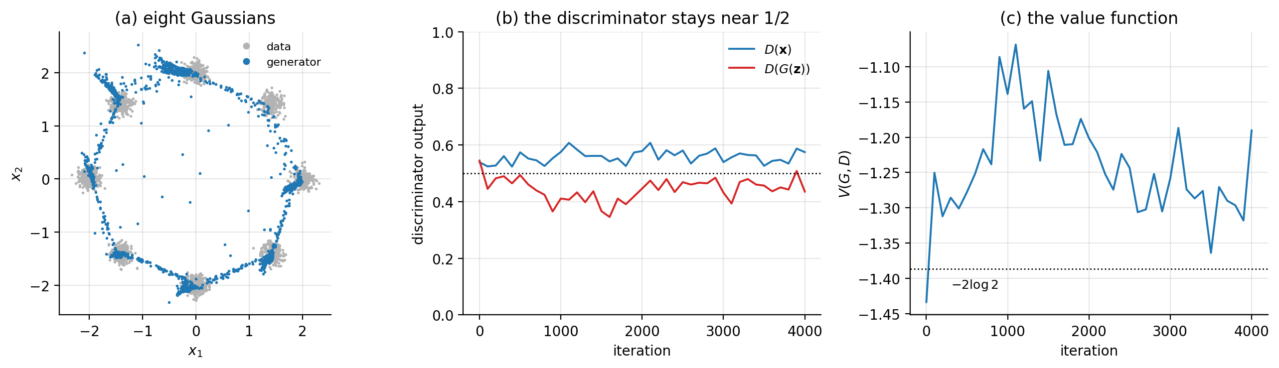
Figure 17.2: A non-saturating GAN on a mixture of eight Gaussians, trained for \(4000\) alternating steps. (a) Data and generated samples; all eight modes are covered, with \(86\%\) of samples within \(0.5\) of a mode centre and the remainder strung along the connecting filaments discussed in Proposition 17.5. (b) \(D(\bm{x})\) and \(D(G(\bm{z}))\) against iteration; both hover around the equilibrium value \(\tfrac{1}{2}\) of Theorem 17.3 without settling on it. (c) The value function \(V(G,D)\) against the predicted \(-2\log2=-1.386\).
17.6. What actually goes wrong#
GAN training is notoriously unstable, and the instability is not a matter of insufficient tuning. Three distinct failure mechanisms operate, and it is worth separating them because they have different remedies.
17.6.1. Non-convergence: the game itself#
The pair \((G^{*},D^{*})\) of Theorem 17.3 is a Nash equilibrium: neither player can improve unilaterally. Gradient descent-ascent, however, is not an algorithm for finding Nash equilibria, and the difference is not subtle. The cleanest demonstration is the smallest possible zero-sum game,
with \(x\) minimising and \(y\) maximising. The unique Nash equilibrium is the origin. Simultaneous gradient updates give
whose matrix has eigenvalues \(1\pm i\gamma\) of modulus \(\sqrt{1+\gamma^{2}}>1\). The iteration therefore spirals outward, and does so exactly:
No step size helps; smaller \(\gamma\) only slows the divergence.
Now alternate, using the updated \(x\) in the \(y\) update as every practical implementation does:
The determinant is \(1-\gamma^{2}+\gamma^{2}=1\) and the trace is \(2-\gamma^{2}\), so for \(\gamma<2\) the eigenvalues are complex conjugates on the unit circle: the orbit neither converges nor diverges but circulates forever at constant radius. Both statements are exact and both are checked:
=== 7. the bilinear game V(x,y) = xy, unique Nash at the origin ===
  gamma   steps    ||(x,y)|| simultaneous (1+gamma^2)^(T/2)    ||(x,y)|| alternating
   0.10    1000             2.0474e+02         2.0474e+02             1.399261
   0.05    1000             4.9284e+00         4.9284e+00             1.411927
   0.01    1000             1.4867e+00         1.4867e+00             1.412129
The starting point has \(\|(x_0,y_0)\|=\sqrt2=1.41421\), and the alternating iteration is still within \(1.1\%\) of it after a thousand steps, while the simultaneous one at \(\gamma=0.1\) has grown by a factor of \(145\). This single \(2\times2\) example explains two facts about GAN practice at once: why the updates are alternated rather than simultaneous, and why even then the loss curves oscillate instead of descending. A GAN is not minimising anything; it is orbiting.
The standard stabilisers all attack this. Setting Adam’s \(\beta_1=0.5\) instead of \(0.9\) reduces the momentum that turns a circulating orbit into an expanding one. Two-time-scale updates [heusel2017] (\(\gamma_d>\gamma_g\)) keep the discriminator closer to its optimum, which is where the theory of Section The objective is a Jensen-Shannon divergence lives. Spectral normalisation bounds the Lipschitz constant of \(D\) [miyato2018], damping the feedback. None of them makes the game convex.
17.6.2. Vanishing gradients: the discriminator wins#
The second mechanism was derived in Section The non-saturating generator loss. If \(D\) becomes perfect – \(D(\bm{x})=1\) on data, \(D(G(\bm{z}))=0\) on samples – then \(V\) is at its ceiling and, with the saturating loss, the generator receives nothing. The non-saturating loss removes the symptom, but the underlying condition is real: a discriminator that separates the two distributions perfectly has, by Eq. (17.9), an infinite logit, and its gradient carries no information about how far the generator is from the data, only that it is on the wrong side. This is the failure the Wasserstein critic of Section The Wasserstein distance is designed to remove at the source.
17.6.3. Mode collapse, and a topological obstruction#
The third mechanism is the one peculiar to adversarial training. In mode collapse the generator maps many different \(\bm{z}\) to the same, or very nearly the same, output. The mechanism is easy to see from the alternating algorithm: for a fixed discriminator the generator’s optimal response is to place all its mass at \(\mathop{\mathrm{arg\,max}}_{\bm{x}}D(\bm{x})\) – a single point – because Eq. (17.20) contains nothing that rewards diversity. The discriminator then learns to reject that point, the generator moves to the next best one, and the pair cycles. The theory of Section The objective is a Jensen-Shannon divergence does not apply, because it assumed \(D=D^{*}\), and \(D^{*}\) would penalise the collapse immediately.
It is instructive to try to provoke it. We use the standard benchmark, a \(5\times5\) grid of narrow Gaussians, and run three objectives:
=== 3. mode collapse: a 5x5 grid of narrow modes ===
  objective              time   modes  in-mode   energy dist  min/max per mode
  non-saturating           46s   15/25    52.4%      0.08026      0 /  354
  strong discriminator     25s   16/25    53.3%      0.12127      2 /  482
  WGAN-GP                 159s   17/25    46.1%      0.02638      3 /  349
  a uniform generator would put 200 of the 5000 samples on each mode
None of the three covers the target. The non-saturating GAN reaches fifteen of the twenty-five modes and puts \(354\) of five thousand samples on its favourite and none at all on its least favourite; strengthening the discriminator makes the imbalance worse, not better, and drives the energy distance up by half. WGAN-GP reaches seventeen modes and cuts the energy distance by a factor of three, which is a real improvement, but it too is far from uniform. Figure 17.4 shows the full distribution of samples over modes for the three runs. We report the failure rather than tuning until it goes away, because the shape of the failure is more informative than a successful run would be.
Look at Figure 17.3. The generated samples do not sit on twenty-five islands: they lie along connected filaments that thread through the modes and, in the outer runs, trace the boundary of the square. This is not an accident of optimisation but a constraint that no amount of training can remove.
Proposition 17.5 (The support of \(p_g\) is connected)
Let \(G:\mathbb{R}^{k}\to\mathbb{R}^{d}\) be continuous and let \(p_z\) have connected support \(S_z\). Then \(G(S_z)\) is connected, and \(\mathrm{supp}(p_g)=\overline{G(S_z)}\) is connected.
Proof
The continuous image of a connected set is connected, and the closure of a connected set is connected.
A Gaussian or uniform prior has connected support and a neural network is continuous, so \(p_g\) is supported on a connected set no matter what the parameters are. If \(p_r\) is supported on twenty-five disjoint islands, the two supports cannot coincide: the generator must either miss modes or connect them with filaments carrying mass the data do not have. It does both, and Figure 17.3 is a picture of the compromise. Real image manifolds are not literally disconnected, but they are close enough to it – a picture halfway between a \(3\) and an \(8\) is not a digit – that the same tension appears, and it is one reason samples from a GAN occasionally look like a blend of two classes.
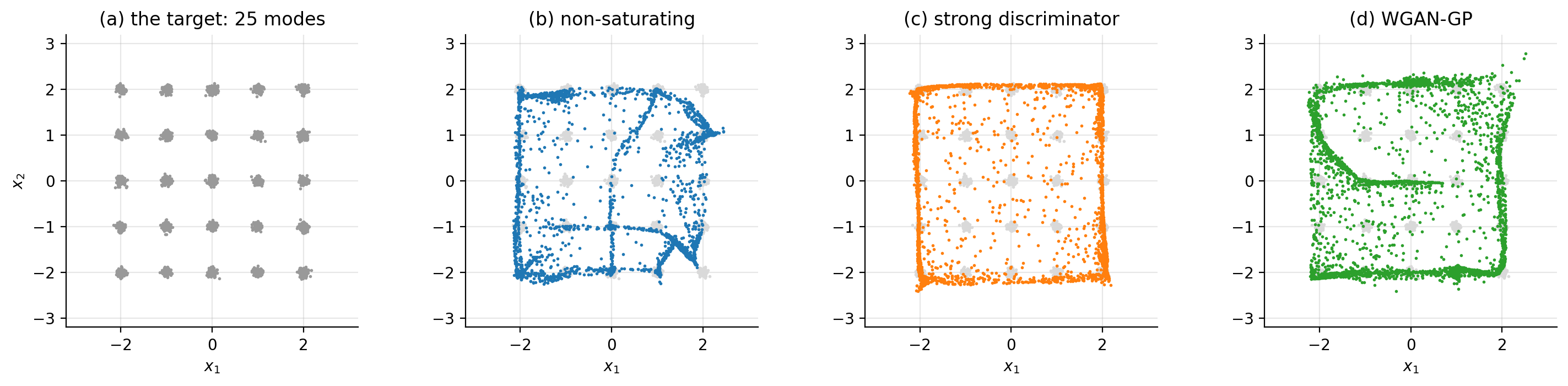
Figure 17.3: Mode collapse on a \(5\times5\) grid of narrow Gaussians. (a) The target. (b) The non-saturating GAN after \(8000\) steps: fifteen of the twenty-five modes are visited, and the samples lie along connected curves rather than on islands. (c) The same with a wider discriminator, a larger discriminator learning rate and three discriminator steps per generator step: the imbalance is worse and the energy distance rises from \(0.080\) to \(0.121\). (d) WGAN-GP, which reaches seventeen modes and an energy distance of \(0.026\). The filaments in all three panels are forced by Proposition 17.5.
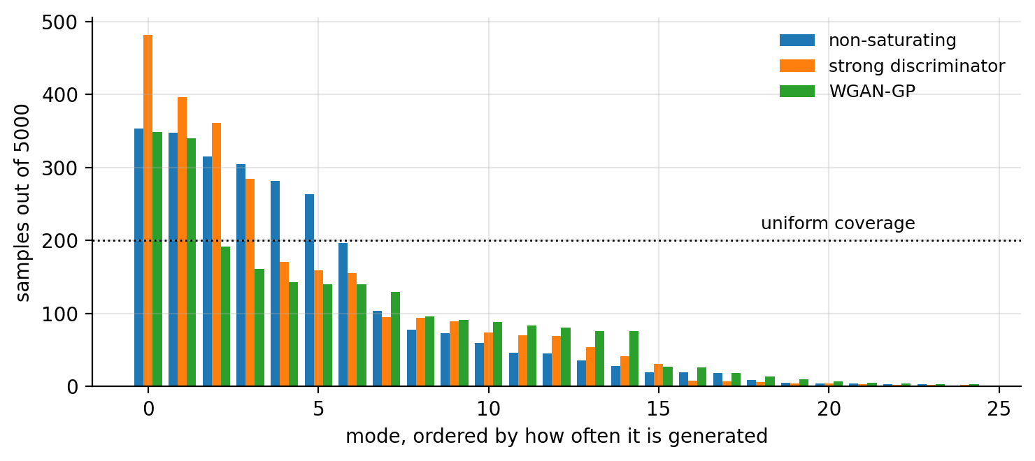
Figure 17.4: How the five thousand generated samples of Figure 17.3 are distributed over the twenty-five modes, sorted from most to least visited for each objective. A generator matching the target would produce the flat line at \(200\). All three are far from it; WGAN-GP is flattest in the tail, which is what its lower energy distance is measuring.
The standard mitigations follow the diagnosis. Minibatch discrimination gives the discriminator access to statistics across a batch rather than single samples, so that a batch of near-identical outputs is detectable and punishable. Unrolled GANs [metz2017] differentiate the generator loss through several future discriminator updates, so that \(G\) cannot exploit a short-sighted \(D\). Spectral normalisation [miyato2018] and the gradient penalty of Section The Wasserstein distance bound the discriminator’s Lipschitz constant. Raising \(k\), the latent dimension, does not help: it cannot change Proposition 17.5, and in our experiments \(k=16\) was measurably worse than \(k=2\).
17.7. The Wasserstein distance#
Lemma 17.2 contains a warning that Section Vanishing gradients: the discriminator wins only hinted at. If \(p_r\) and \(p_g\) have disjoint supports, then \(D_{\mathrm{JS}}(p_r\|p_g)=\log2\) exactly, whatever the distance between the supports. By Theorem 17.3 the objective is then flat: its gradient with respect to any parameter of \(G\) that moves \(p_g\) without creating overlap is zero.
This is not a pathological case. A generator maps a \(k\)-dimensional latent into \(\mathbb{R}^{d}\) with \(k\ll d\), so \(p_g\) is supported on a manifold of dimension at most \(k\); the data lie on their own low-dimensional manifold; two such manifolds in general position intersect in a set of measure zero. Early in training the supports are effectively disjoint, and the ideal objective offers no guidance at all.
The canonical illustration is one-dimensional. Let \(p_r\) be uniform on \([0,1]\) and \(p_g\) uniform on \([\theta,\theta+1]\). The overlap has length \((1-\theta)_+\); on it both densities are \(1\) and the mixture is also \(1\), so that region contributes nothing to Eq. (17.11); off it exactly one density is \(1\) while the mixture is \(\tfrac12\), contributing \(\log2\) per unit length. Hence
For \(\theta\ge1\) the divergence is pinned at \(\log2\) with zero derivative, while the Wasserstein distance defined below keeps a derivative of \(1\) everywhere. Figure 17.5 plots both, together with the Gaussian case computed by quadrature:
=== 6b. JS and W for two unit Gaussians, by quadrature ===
       mu       JS(N(0,1)||N(mu,1))      W = |mu|
      0.50            0.03031130          0.5000
      1.00            0.11142148          1.0000
      2.00            0.33683082          2.0000
      4.00            0.63272019          4.0000
      8.00            0.68516989          8.0000
Gaussians have full support, so the divergence never quite reaches \(\log2\); but at \(\mu=8\) it is within \(0.008\) of the ceiling and for practical purposes the gradient is gone.
The Wasserstein-1 or earth-mover distance measures how far mass must be moved rather than how much the densities disagree:
where \(\Pi(p_r,p_g)\) is the set of joint distributions – transport plans – with the prescribed marginals. The infimum over plans is intractable, but the Kantorovich-Rubinstein duality [villani2009] converts it into a maximisation over functions,
the supremum running over all \(1\)-Lipschitz \(f\). This is a form we can parameterise: replace \(f\) by a network \(f_w\), drop the sigmoid – the output is no longer a probability, which is why \(f_w\) is called a critic rather than a discriminator – and maximise Eq. (17.28) by gradient ascent.
The Lipschitz constraint is the whole difficulty. The original WGAN [arjovsky2017] clipped every weight to \([-c,c]\), which enforces some Lipschitz bound but also cripples the critic’s capacity. The gradient penalty [gulrajani2017] replaces the hard constraint by a soft one, using the fact that a differentiable function is \(1\)-Lipschitz if and only if \(\|\nabla f\|\le1\) everywhere, and that the optimal critic in Eq. (17.28) has \(\|\nabla f\|=1\) almost everywhere on the transport paths. Sampling those paths by interpolating between real and generated points gives
with \(\hat{\bm{x}}=\epsilon\bm{x}+(1-\epsilon)G(\bm{z})\), \(\epsilon\sim U[0,1]\) and \(\lambda=10\) the standard choice. The generator maximises \(\mathbb{E}[f_w(G(\bm{z}))]\). Because the critic is now expected to be trained close to its optimum, \(n_{\mathrm{critic}}=5\) is used instead of \(1\).
Two practical differences follow. The critic loss is an estimate of \(W\) up to a constant, so unlike \(V\) it decreases as the samples improve and is usable as a progress indicator; and batch normalisation must be removed from the critic, since the penalty is a statement about the gradient with respect to a single input and batch normalisation makes the output depend on the whole batch. In our two-dimensional experiment WGAN-GP gave the lowest energy distance of the three objectives, \(0.026\) against \(0.080\), at four times the cost in wall-clock time. The implementation is short:
def gradient_penalty(Q, x_real, x_fake, rng):
    """E[(||grad f_w(xhat)||_2 - 1)^2] on the segments between real and fake."""
    eps = rng.uniform(0.0, 1.0, (len(x_real), 1))
    xhat = eps * x_real + (1.0 - eps) * x_fake
    g = grad(lambda x: np.sum(critic(Q, x)))(xhat)
    return np.mean((np.sqrt(np.sum(g ** 2, axis=1) + 1e-12) - 1.0) ** 2)


def critic_loss(Q, P, x_real, z, rng, lam=10.0):
    """L_critic = E_pg[f] - E_pr[f] + lambda * GP,  Eq. (17.wgangp)."""
    x_fake = generator(P, z)
    w = np.mean(critic(Q, x_fake)) - np.mean(critic(Q, x_real))
    return w + lam * gradient_penalty(Q, x_real, x_fake, rng)
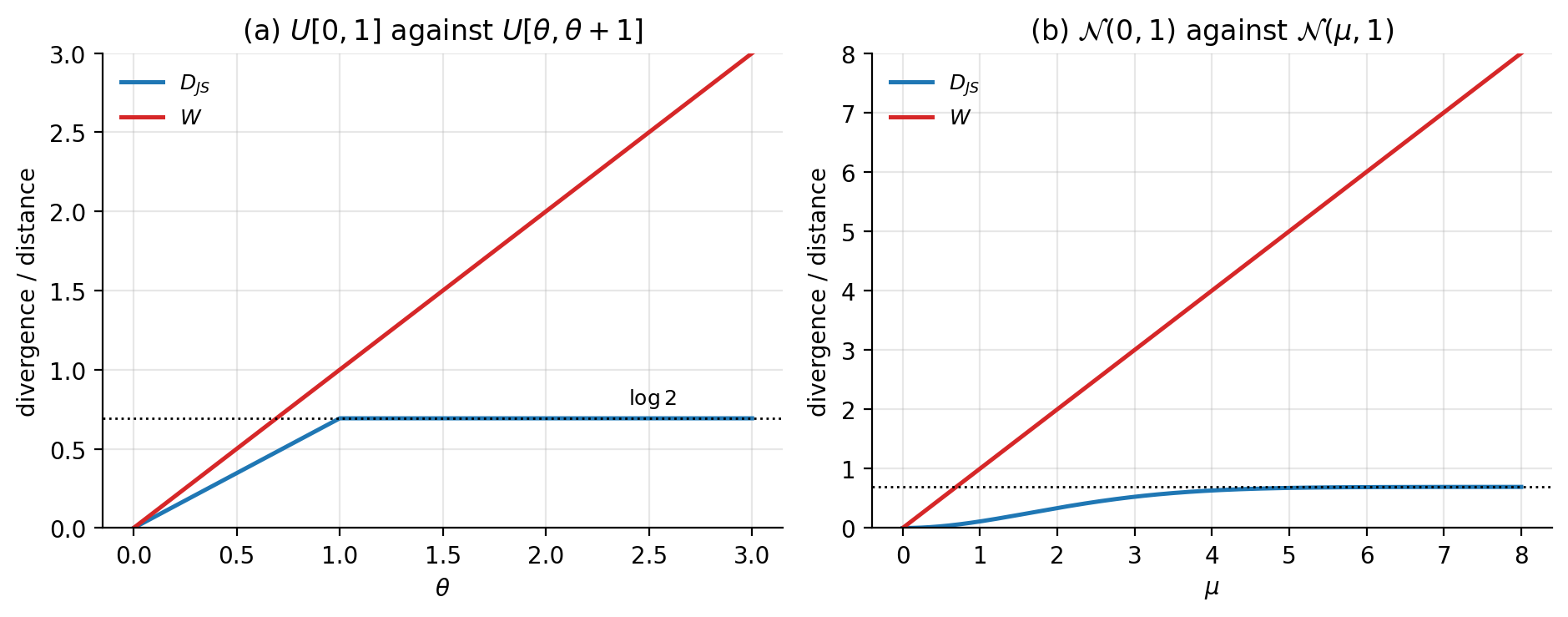
Figure 17.5: Why the Jensen-Shannon divergence gives up. (a) \(p_r=U[0,1]\) against \(p_g=U[\theta,\theta+1]\): Eq. (17.26) makes \(D_{\mathrm{JS}}\) constant at \(\log2\) for \(\theta\ge1\), so the objective has no gradient there, while \(W=\theta\) has slope \(1\) everywhere. (b) The same comparison for \(\mathcal{N}(0,1)\) against \(\mathcal{N}(\mu,1)\), computed by quadrature: the supports overlap so \(D_{\mathrm{JS}}\) approaches \(\log2\) asymptotically instead of reaching it, but by \(\mu=4\) it is already within \(0.06\) of the ceiling.
17.8. Evaluating a model with no likelihood#
Every generative model of the preceding chapters could be scored on held-out data by its likelihood or a bound on it. A GAN offers neither, and the question “is this model better than that one?” has to be answered from samples alone. Three families of answer are in use.
17.8.1. Maximum mean discrepancy#
Given a kernel \(k(\cdot,\cdot)\), the maximum mean discrepancy [gretton2012] between \(p\) and \(q\) is the distance between their mean embeddings in the corresponding reproducing kernel Hilbert space,
For a characteristic kernel – the Gaussian \(k(\bm{x},\bm{y})=\exp(-\|\bm{x}-\bm{y}\|^{2}/2\sigma^{2})\) is one – the mean embedding determines the distribution, so \(\mathrm{MMD}(p,q)=0\) if and only if \(p=q\). With \(n\) real and \(m\) generated samples the unbiased estimator omits the diagonal terms,
because \(k(\bm{x}_i,\bm{x}_i)=1\) contributes a bias of order \(1/n\) that does not cancel between the three terms. The energy distance used throughout this chapter is the same construction with the conditionally negative definite kernel \(-\|\bm{x}-\bm{y}\|\):
which needs no bandwidth to be chosen and is what makes it convenient for the two-dimensional experiments here. In high dimensions the choice of \(\sigma\) in Eq. (17.30) matters a great deal, which is the practical objection to MMD on images.
17.8.2. Fr’echet inception distance#
The most widely reported metric [heusel2017] sidesteps the kernel choice by working in the feature space of a fixed pretrained classifier. Push \(n\) real and \(n\) generated images through the penultimate layer of an InceptionV3 network, fit a Gaussian to each set of feature vectors, and report the Fr’echet distance between the two Gaussians:
Equation (17.33) is not an arbitrary formula: it is exactly the squared \(2\)-Wasserstein distance between two Gaussians, so FID is \(W_2^{2}\) computed in feature space under a Gaussian approximation. The connection to Section The Wasserstein distance is therefore closer than it looks – the metric of choice for evaluating GANs is a Wasserstein distance, in a space where the disjoint-support problem has been removed by the feature map.
Lower is better. The caveats are that FID depends on the feature extractor, that it is biased at small \(n\) (ten thousand samples is the usual minimum because \(\bm{\Sigma}\) is a \(2048\times2048\) matrix), and that a Gaussian is a crude model of the feature distribution. The older inception score, \(\exp\bigl(\mathbb{E}_{\bm{x}}D_{\mathrm{KL}}(p(y|\bm{x})\|p(y))\bigr)\), rewards confident and diverse classifications but never looks at the real data at all, and is correspondingly easy to fool.
No metric detects mode collapse reliably
A generator that reproduces one mode perfectly can achieve a respectable FID, because the Gaussian fit in Eq. (17.33) is dominated by the mean and the bulk of the covariance. This is why the experiments of Section Mode collapse, and a topological obstruction count modes explicitly, which is possible only because the target was constructed. For real data the honest procedures are precision-recall curves, which separate fidelity from coverage instead of averaging them, and looking at a large grid of samples. A single number that summarises a distribution will always be able to hide something.
17.9. Architectures#
The theory above says nothing about how \(G\) and \(D\) are built, and in practice the architecture matters as much as the loss.
17.9.1. The fully connected baseline#
For MNIST the original recipe is a pair of multilayer perceptrons,
with the generator using batch normalisation and LeakyReLU\((0.2)\) after each linear layer and \(\tanh\) at the output, and the discriminator mirroring it without batch normalisation and with dropout. Four conventions in that sentence deserve their reasons:
\(\tanh\) at the generator output, with the data rescaled to \([-1,1]\). A bounded output prevents the generator from escaping to large values when the discriminator is briefly weak.
LeakyReLU rather than ReLU, in both networks. A dead ReLU unit in \(D\) contributes no gradient to \(G\) either, and the adversarial game provides plenty of opportunity for units to die.
Batch normalisation in \(G\) but not in \(D\). In \(D\) it makes the verdict on one sample depend on the rest of the batch, which is both a leak of information and a source of instability; in \(G\) it keeps activations scaled while the target distribution moves.
Adam with \(\beta_1=0.5\) and \(\gamma=2\times10^{-4}\). The reduced momentum is the practical response to Eq. (17.23).
17.9.2. Convolutions: DCGAN#
The deep convolutional GAN of Radford, Metz and Chintala [radford2016] replaced the fully connected layers with strided convolutions: fractionally strided (transposed) convolutions in \(G\) to upsample from \(\bm{z}\) to an image, ordinary strided convolutions in \(D\) to downsample, no pooling anywhere, and no fully connected layers except the projection of \(\bm{z}\). Weights are initialised from \(\mathcal{N}(0,0.02^{2})\). These conventions are still the default starting point, and the architectural reason is the one from Chapter 10: the convolutional prior of locality and weight sharing is right for images, and a generator that must learn translation equivariance from scratch wastes its capacity on it.
17.9.3. Conditioning#
A conditional GAN [mirza2014] gives both networks a side input \(\bm{y}\) – a class label, a segmentation map, a text embedding:
The analysis is unchanged: conditioning on \(\bm{y}\) and applying Proposition 17.1 pointwise in \(\bm{x}\) for each fixed \(\bm{y}\) gives
and Theorem 17.3 becomes a statement about the expectation over \(\bm{y}\) of the conditional divergences, \(\mathbb{E}_{\bm{y}}\bigl[D_{\mathrm{JS}}(p_r(\cdot|\bm{y})\|p_g(\cdot|\bm{y}))\bigr]\). For MNIST, \(\bm{y}\) is a one-hot vector in \(\mathbb{R}^{10}\) concatenated to \(\bm{z}\) and, as an extra channel or an extra input vector, to \(\bm{x}\). Conditioning is what turns a GAN from a curiosity into a tool: image-to-image translation, super-resolution and text-to-image synthesis are all Eq. (17.35) with different \(\bm{y}\).
17.9.4. Reading the latent space#
A trained generator can be probed by interpolating between two noise vectors. Linear interpolation,
is the obvious choice and it is wrong, for a reason worth computing. For \(\bm{z}\sim\mathcal{N}(\bm{0},\bm{I}_k)\) we have \(\mathbb{E}\|\bm{z}\|^{2}=k\), and the norm concentrates: its standard deviation tends to \(1/\sqrt2\) independently of \(k\). The midpoint of two independent draws has
so its norm is smaller by \(\sqrt2\). For \(k=100\) that is a shift from \(10\) to \(7.07\), some four standard deviations inward – a region from which the prior essentially never draws and on which the generator has therefore never been trained. Measured:
=== 8. the norm of a Gaussian latent vector ===
      k     E||z||    sd(||z||)   E||(z1+z2)/2||   sqrt(k/2)   deviation in sd
      2     1.2532      0.6537          0.8861      1.0000             0.6
     16     3.9372      0.7026          2.7835      2.8284             1.6
    100     9.9754      0.7049          7.0539      7.0711             4.1
The remedy is to interpolate along the sphere the prior actually occupies,
which preserves the norm when \(\|\bm{z}_1\|=\|\bm{z}_2\|\) and reduces to Eq. (17.37) as \(\Omega\to0\). A smooth transition under Eq. (17.39) is evidence that the generator has learned a coherent manifold; abrupt jumps indicate that it has memorised a few outputs. It is a qualitative test, but it detects things FID does not.
\noalign{} Variant |
Change |
Objective |
What it buys |
|---|---|---|---|
\noalign{}\noalign{} GAN |
– |
\(D_{\mathrm{JS}}\), Eq. (17.12) |
the construction |
Non-sat. |
\(-\log D(G(\bm{z}))\) |
same fixed point |
gradients when losing |
cGAN |
side input \(\bm{y}\) |
conditional \(D_{\mathrm{JS}}\) |
control |
WGAN |
critic, weight clipping |
\(W\), Eq. (17.28) |
gradients on disjoint supports |
WGAN-GP |
gradient penalty |
Eq. (17.29) |
Lipschitz without clipping |
DCGAN |
strided convolutions |
any of the above |
images |
StyleGAN [karras2019] |
style-modulated generator |
any of the above |
control of scale-wise detail |
\noalign{} |
Table 17.1: The main variants. All but the last two rows differ only in the loss or the conditioning; the architecture rows change what the networks are made of.
17.10. GANs in PyTorch and TensorFlow#
The two-dimensional programs above were written with explicit gradients so that the two players could be seen separately. In a library the same structure appears as two optimisers and one detach. Here is the PyTorch version of the architectures of Section The fully connected baseline; note that the discriminator returns a logit, so that \verb!BCEWithLogitsLoss! can apply the sigmoid internally and the losses of Eqs. (17.17) and (17.20) are evaluated stably:
import torch
import torch.nn as nn


def make_generator_fc(k_z=100, n_out=784, widths=(256, 512, 1024)):
    """z in R^k -> image in [-1,1]^784, Eq. (17.generator)."""
    layers, n_in = [], k_z
    for w in widths:
        layers += [nn.Linear(n_in, w), nn.BatchNorm1d(w),
                   nn.LeakyReLU(0.2, inplace=True)]
        n_in = w
    layers += [nn.Linear(n_in, n_out), nn.Tanh()]
    return nn.Sequential(*layers)


def make_discriminator_fc(n_in=784, widths=(1024, 512, 256), p_drop=0.3):
    """image -> logit u(x); D(x) = sigmoid(u(x)).  No batch norm in D."""
    layers = []
    for w in widths:
        layers += [nn.Linear(n_in, w), nn.LeakyReLU(0.2, inplace=True),
                   nn.Dropout(p_drop)]
        n_in = w
    layers += [nn.Linear(n_in, 1)]
    return nn.Sequential(*layers)
The training step is the algorithm of Section Training: alternating gradients written out. The single most important line is \verb!.detach()!: without it the discriminator update would also send gradients backwards into the generator, which is not what Eq. (17.15) says.
G, D = make_generator_fc(), make_discriminator_fc()
opt_g = torch.optim.Adam(G.parameters(), lr=2e-4, betas=(0.5, 0.999))
opt_d = torch.optim.Adam(D.parameters(), lr=2e-4, betas=(0.5, 0.999))
bce = nn.BCEWithLogitsLoss()

for x, _ in loader:                            # x in [-1,1], flattened
    n = x.size(0)

    # --- discriminator: gradient ascent on V, Eq. (17.dstep) --------------
    z = torch.randn(n, 100)
    x_fake = G(z).detach()                     # no gradient into G here
    u_real, u_fake = D(x), D(x_fake)
    loss_d = (bce(u_real, torch.full_like(u_real, smooth))   # smooth = 1.0 or 0.9
              + bce(u_fake, torch.zeros_like(u_fake)))       # Eq. (17.dloss)
    opt_d.zero_grad(set_to_none=True)
    loss_d.backward()
    opt_d.step()

    # --- generator: non-saturating loss, Eq. (17.nonsat) ------------------
    z = torch.randn(n, 100)
    loss_g = bce(D(G(z)), torch.ones(n, 1))    # = -log D(G(z))
    opt_g.zero_grad(set_to_none=True)
    loss_g.backward()
    opt_g.step()
The gradient penalty of Eq. (17.29) needs a derivative with respect to an input, which is why \verb!create_graph=True! appears: the penalty is itself differentiated when the critic is updated.
def gradient_penalty(D, x_real, x_fake):
    eps = torch.rand(x_real.size(0), *([1] * (x_real.dim() - 1)))
    xhat = (eps * x_real + (1 - eps) * x_fake).requires_grad_(True)
    g = torch.autograd.grad(D(xhat).sum(), xhat, create_graph=True)[0]
    return ((g.flatten(1).norm(2, dim=1) - 1.0) ** 2).mean()
The TensorFlow version is the same algorithm with different bookkeeping. PyTorch accumulates gradients on the parameters and we zero them; TensorFlow records a tape and we ask it for the gradient of one loss with respect to one list of variables. The two tapes are the two players:
import tensorflow as tf
from tensorflow import keras
from tensorflow.keras import layers

bce = keras.losses.BinaryCrossentropy(from_logits=True)


def make_generator_fc(k_z=100, n_out=784, widths=(256, 512, 1024)):
    m = keras.Sequential([keras.Input(shape=(k_z,))])
    for w in widths:
        m.add(layers.Dense(w, use_bias=False))
        m.add(layers.BatchNormalization())
        m.add(layers.LeakyReLU(negative_slope=0.2))
    m.add(layers.Dense(n_out, activation="tanh"))
    return m


def make_discriminator_fc(n_in=784, widths=(1024, 512, 256), p_drop=0.3):
    m = keras.Sequential([keras.Input(shape=(n_in,))])
    for w in widths:
        m.add(layers.Dense(w))
        m.add(layers.LeakyReLU(negative_slope=0.2))
        m.add(layers.Dropout(p_drop))
    m.add(layers.Dense(1))                     # a logit, not a probability
    return m


G, D = make_generator_fc(), make_discriminator_fc()
opt_g = keras.optimizers.Adam(2e-4, beta_1=0.5)
opt_d = keras.optimizers.Adam(2e-4, beta_1=0.5)


@tf.function
def train_step(x, k_z=100, smooth=1.0):
    n = tf.shape(x)[0]

    # --- discriminator ----------------------------------------------------
    x_fake = G(tf.random.normal([n, k_z]), training=True)   # outside the tape
    with tf.GradientTape() as tape:                         # = detach()
        u_real, u_fake = D(x, training=True), D(x_fake, training=True)
        loss_d = (bce(tf.fill(tf.shape(u_real), smooth), u_real)
                  + bce(tf.zeros_like(u_fake), u_fake))
    opt_d.apply_gradients(zip(tape.gradient(loss_d, D.trainable_variables),
                              D.trainable_variables))

    # --- generator, Eq. (17.nonsat) ---------------------------------------
    with tf.GradientTape() as tape:
        u_fake = D(G(tf.random.normal([n, k_z]), training=True), training=True)
        loss_g = bce(tf.ones_like(u_fake), u_fake)
    opt_g.apply_gradients(zip(tape.gradient(loss_g, G.trainable_variables),
                              G.trainable_variables))
    return loss_d, loss_g, tf.sigmoid(u_real), tf.sigmoid(u_fake)
In both frameworks the quantities to watch during training are not the losses – which oscillate, by Section Non-convergence: the game itself – but the mean of \(D(\bm{x})\) and of \(D(G(\bm{z}))\). Theorem 17.3 says both should approach \(\tfrac12\). If \(D(G(\bm{z}))\) collapses towards zero the discriminator is winning and the generator is starving; if \(D(\bm{x})\) falls towards \(\tfrac12\) while \(D(G(\bm{z}))\) rises above it, the discriminator has been overwhelmed and its gradient is no longer informative. Both are reasons to stop, and neither is visible in the loss curves.
When to stop
There is no early-stopping criterion for a GAN, because there is no held-out score that decreases monotonically. The practical procedure is to save samples on a fixed noise batch \(\bm{z}_{\mathrm{fixed}}\) at every epoch – as both programs do – and to select the epoch afterwards, by FID if the domain has a trusted feature extractor and by eye if not. Keeping the noise fixed matters: it separates changes in the generator from changes in the sample.
17.11. Summary and the programs#
A generative adversarial network replaces the likelihood by a classifier. The classifier’s optimum, Proposition 17.1, is the density ratio \(p_r/(p_r+p_g)\) in disguise, verified here to \(3\times10^{-9}\) pointwise and to \(0.024\) rms by a trained network wherever data exist – and badly violated where they do not, which is Figure 17.1(b) and the first warning of the chapter. Substituting that optimum back, the generator turns out to be minimising a Jensen-Shannon divergence, Theorem 17.3, confirmed against quadrature to \(10^{-12}\), with the global minimum \(-2\log2\) attained exactly when \(p_g=p_r\) and \(D\equiv\tfrac12\).
That is the theory, and the rest of the chapter is the distance between it and the algorithm. The saturating loss of Eq. (17.4) starves the generator by a factor \((1-D)/D\), Eq. (17.19), which we measured growing to \(23\) while the discriminator trained alone; the non-saturating loss of Eq. (17.20) fixes it without moving the fixed point. Label smoothing caps the discriminator at \(s\), Proposition 17.4, and was measured holding \(D(\bm{x})\) down to \(0.86\) instead of \(0.97\). Alternating gradient updates do not converge to a Nash equilibrium: on the bilinear game the simultaneous iteration diverges exactly as \((1+\gamma^{2})^{t/2}\) and the alternating one circulates forever, both confirmed to five figures, which is why our trained GAN sat at \(V=-1.275\) rather than \(-1.386\) and why the loss curves of any GAN oscillate.
Two limitations are structural rather than numerical. The Jensen-Shannon divergence is pinned at \(\log2\) on disjoint supports, Lemma 17.2, so early training has no gradient at all in the idealised objective; the Wasserstein distance of Eq. (17.28) with the gradient penalty of Eq. (17.29) repairs this, and cut the energy distance on our benchmark from \(0.080\) to \(0.026\) at four times the cost. And the support of \(p_g\) is connected whatever the parameters, Proposition 17.5, so a disconnected target cannot be matched: none of our three objectives covered more than seventeen of twenty-five modes, and all three produced the connecting filaments of Figure 17.3.
What is bought with all this is a generator that produces sharp samples in a single forward pass, with no bound, no partition function and no iterative sampler – and an evaluation problem, since with no likelihood the only available scores are two-sample statistics, Eqs. (17.30) and (17.33), none of which reliably detects the mode collapse the method is prone to.
The programs are in the directory
doc/BookML/BookPrograms/chapter17_gan.
Every listing above appears there, and five modules run start to finish and reproduce the numbers quoted in the text:
gan.py– the networks, the three generator losses of Section The non-saturating generator loss, the gradient penalty of Eq. (17.29), Adam with \(\beta_1=0.5\), the alternating training loop, and the two-dimensional targets.verify_gan.py– the eight checks: the pointwise optimum, the trained discriminator against Eq. (17.6), the Jensen-Shannon identity, label smoothing, the two generator gradients, the failure of \(D_{\mathrm{JS}}\) on disjoint supports, the bilinear game, and the geometry of the Gaussian prior.run_compare.py– the equilibrium experiment of Section What convergence looks like, the gradient-starvation experiment of Section The non-saturating generator loss, and the mode-collapse comparison of Section Mode collapse, and a topological obstruction.gan_torch.py– the MNIST program in PyTorch, with the fully connected and DCGAN architectures and the non-saturating, saturating and WGAN-GP losses selectable from the command line.gan_tf.py– the same program in TensorFlow.
The figures are generated by ch17_figures.py in
doc/BookML/BookFigures; none is drawn by hand.
17.12. Exercises#
17.12.1. Warm-up exercises#
The optimal discriminator. (a) Derive Eq. (17.6) by differentiating \(f(t)=A\log t+B\log(1-t)\) and verify with Eq. (17.8) that it is a maximum and not a minimum. (b) What is \(D^{*}\) at a point where \(p_r>0\) but \(p_g=0\), and what does the generator learn there? (c) Show that the logit of \(D^{*}\) is the log density ratio, Eq. (17.9), and explain why this makes \(D^{*}\) a substitute for a likelihood.
Bounds on the Jensen-Shannon divergence. Prove Lemma 17.2 and state the conditions for equality at each end. Then compute \(D_{\mathrm{JS}}\) for two Bernoulli distributions with parameters \(p\) and \(q\) and plot it; where is it steepest?
Vanishing gradients. At \(D(G(\bm{z}))=\varepsilon\ll1\), compute the magnitude of the generator gradient for the saturating and the non-saturating losses and confirm Eq. (17.19). Then explain why the measured ratio in Section The non-saturating generator loss was \(23\) when \(1/D(G(\bm{z}))\) was \(41.5\).
Label smoothing. (a) Derive Proposition 17.4. (b) Repeat the derivation smoothing both labels, real to \(s\) and generated to \(\varepsilon>0\), and show that the optimum becomes \(\bigl(sp_r+\varepsilon p_g\bigr)/(p_r+p_g)\). Explain from this expression why two-sided smoothing is a bad idea.
Wasserstein against Jensen-Shannon. (a) Derive Eq. (17.26) for the two uniform distributions. (b) Show that \(W(\mathcal{N}(0,1),\mathcal{N}(\mu,1))=|\mu|\), using the fact that in one dimension the optimal transport plan matches quantiles. (c) Which of the two has a useful gradient at \(\mu=10\)?
The bilinear game. Verify the eigenvalues quoted for Eqs. (17.23) and (17.25), derive Eq. (17.24), and show that the alternating iteration conserves a quadratic form. What does this conserved quantity correspond to in a real GAN?
Counting. A GAN, a VAE and a diffusion model with \(T=1000\) each generate one image. How many network evaluations does each need? How many does each need to evaluate, or bound, \(\log p(\bm{x})\) for a given \(\bm{x}\)?
Conditioning. Derive Eq. (17.36) and state the conditional form of Theorem 17.3. What happens if the generator ignores \(\bm{y}\) entirely – can the discriminator detect it, and if so how?
17.12.2. Project-style exercise: an adversarial generator#
Part a: the theory, numerically. Reproduce the checks of Section The optimal discriminator and Section The objective is a Jensen-Shannon divergence: maximise the integrand pointwise against Eq. (17.6), train a discriminator on two known one-dimensional densities and compare it with the closed form both where the data are and where they are not, and verify Eq. (17.12) against quadrature for several pairs of Gaussians. Report the accuracy you obtain and explain the size of each discrepancy.
Part b: the two losses. Implement both generator losses. Freeze an untrained generator, train the discriminator alone, and plot both generator gradient norms against \(D(G(\bm{z}))\) as in Figure 17.1(c). Then train two full GANs, one with each loss, from the same seed, and compare. Under what conditions does the saturating loss actually fail, and why did it not fail on the eight-Gaussian problem of Section What convergence looks like?
Part c: the equilibrium. Train on the eight-Gaussian mixture and monitor \(D(\bm{x})\), \(D(G(\bm{z}))\) and \(V\). Do they approach the values of Theorem 17.3? Vary the learning-rate ratio \(\gamma_d/\gamma_g\) and \(n_{\mathrm{critic}}\), and report how close to \(-2\log2\) you can get. Then add Adam momentum \(\beta_1=0.9\) and describe what happens in the light of Eq. (17.23).
Part d: mode collapse. Reproduce the \(5\times5\) experiment. Count modes, plot the histogram of Figure 17.4, and try at least three mitigations: minibatch discrimination, one-sided label smoothing, and WGAN-GP. Which helps most, and does any of them beat Proposition 17.5? Test the proposition directly by plotting \(G\) along a straight line in latent space and showing that the output path is continuous.
Part e: Wasserstein. Implement the critic and the gradient penalty of Eq. (17.29). Verify that the penalty really does keep \(\|\nabla f_w\|\) near \(1\) by measuring it on interpolates during training. Compare \(\lambda=0\), \(1\), \(10\) and \(100\), and compare the gradient penalty against weight clipping at several clip values. Does the critic loss track sample quality, as claimed in Section The Wasserstein distance?
Part f: MNIST. Train the fully connected GAN of Section The fully connected baseline on MNIST in PyTorch or TensorFlow, saving samples from a fixed noise batch at every epoch. Then train the DCGAN version and compare. Report FID or, if that is too expensive, MMD in the feature space of a small classifier you train yourself. Show the latent interpolations of Eqs. (17.37) and (17.39) side by side and comment on the difference in the light of Eq. (17.38).
Part g: conditioning. Extend your MNIST GAN to the conditional form of Eq. (17.35) and generate each digit on demand. Then use the conditional generator for data augmentation: train a classifier on \(1000\) real images, and on \(1000\) real images plus generated ones, and report the test accuracy of each. Does the augmentation help, and does the answer depend on how far the generator has been trained?
Part h: a physics application. Train a GAN on configurations of the two-dimensional Ising model at several temperatures, as in part e of the Chapter 14 project, and compare the energy and magnetisation histograms of the generated configurations with the true ones. Then compare against the RBM of Chapter 14 and the diffusion model of Chapter 16 at matched parameter counts. Which reproduces the critical region best, which is fastest to sample, and which would you trust to report an uncertainty? Defend your answer with the divergences of this chapter, not with the pictures.