
7. Chapter 7: Ensemble methods; from simple decision trees to Gradient Boosting#
Every method so far has fitted a single global function to the data: a hyperplane, a sigmoid of a hyperplane, a kernel expansion. Decision trees do something different. They partition the feature space into boxes and fit a constant in each, building the model by a sequence of simple yes-or-no questions. The result is the most interpretable model in this book – a tree can be read aloud – and also, on its own, one of the least accurate.
That combination is what makes the chapter interesting. A single tree has low bias and very high variance, in the sense of Section The bias-variance tradeoff: split the training data in two and fit a tree to each half, and the two trees may look nothing alike. The remedy is to build many trees and combine them, and the various ways of doing so – bagging, random forests, AdaBoost, gradient boosting – are the ensemble methods of the title. They are, on tabular data, the most accurate methods known, and they routinely outperform neural networks in that setting.
We shall build all of them from scratch, because each is short enough to write in a page and because doing so makes the mathematics concrete. Only for XGBoost, in Section XGBoost: extreme gradient boosting, do we use a library – and even there we derive the objective it minimises.
7.1. Basics of a tree#
A decision tree is a sequence of binary questions. The root node contains all the observations; each internal node tests one feature against a threshold and sends the observation left or right; each leaf or terminal node carries a prediction. Classifying or predicting a new point means walking from the root to a leaf, which costs one comparison per level.
Geometrically, each test \(x_j\le t\) cuts the feature space with a hyperplane perpendicular to axis \(j\). A tree therefore partitions the space into axis-aligned boxes, one per leaf, and predicts a constant within each box. This is the central limitation and the central strength: boxes cannot represent a diagonal boundary economically – a tree approximates one by a staircase – but they require no notion of distance, no scaling of the features, and they handle categorical variables and interactions without any special provision.
7.2. Regression trees#
Building a regression tree involves two steps. First we split the predictor space – the set of possible values \(x_1,x_2,\dots,x_p\) – into \(J\) distinct and non-overlapping regions \(R_1,R_2,\dots,R_J\). Second, for every observation falling into region \(R_j\) we make the same prediction, namely the mean of the response values of the training observations in \(R_j\).
In principle the regions could have any shape; we take them to be high-dimensional rectangles, or boxes, for simplicity and for ease of interpretation. The goal is to find boxes minimising
where \(\overline{y}_{R_j}\) is the mean response of the training observations within box \(j\). That the optimal constant in each box is the mean is not an assumption but a consequence: minimising \(\sum_i(y_i-c)^{2}\) over \(c\) gives \(c=\overline{y}\), by the same one-line calculation that produced the sample mean in Section Samples, estimators and their properties.
Recursive binary splitting. It is computationally infeasible to consider every possible partition of the feature space into \(J\) boxes – the number of partitions grows combinatorially – so we proceed top-down and greedily. Top-down because we begin with all observations in a single region and successively split; greedy because at each step we make the best split available at that step, rather than looking ahead to a split that might enable a better one later.
We begin by selecting a predictor \(x_j\) and a cutpoint \(s\) splitting the space into
so as to minimise
searching over all predictors \(x_1,\dots,x_p\) and, for each, over all possible values of \(s\). In practice only \(n-1\) distinct thresholds per feature need be examined – the midpoints between consecutive sorted values – since the criterion is constant between them. The cost of one split is therefore \(\bigO(pn\log n)\) for the sorting, and finding the best \((j,s)\) is quick as long as \(p\) is not enormous.
We then repeat, looking for the best predictor and cutpoint with which to split one of the two regions just created, giving three regions; then split one of those three; and so on, until a stopping criterion is met – commonly that no region contains more than some minimum number of observations.
7.2.1. Cost-complexity pruning#
The procedure above is straightforward but leads to overfitting and to unnecessarily large trees. Grown to completion, a tree places every training point in its own leaf and has zero training error – and, by Section Training error, test error and generalisation, has learned nothing. A smaller tree with fewer splits will have larger bias but smaller variance and better interpretability.
The standard remedy is to grow a large tree \(T_0\) and then prune it back. Rather than considering every subtree, we consider a sequence indexed by a non-negative parameter \(\alpha\), seeking for each \(\alpha\) the subtree \(T\subset T_0\) minimising
where \(\overline{T}\) is the number of terminal nodes and \(R_m\) the region belonging to the \(m\)-th of them.
Equation (7.4) should look familiar: it is a training error plus \(\alpha\) times a complexity penalty, which is precisely the structure of Ridge regression in Eq. (3.43), with the number of leaves playing the role of \(\|\bm{\theta}\|^{2}\). When \(\alpha=0\) the subtree is \(T_0\) itself, since the equation then measures only training error; as \(\alpha\) grows there is an increasing price for many terminal nodes and the minimising subtree shrinks.
It turns out that as \(\alpha\) increases from zero, branches are pruned in a nested and predictable fashion, so the whole sequence of subtrees can be obtained cheaply. We select \(\alpha\) by cross-validation, exactly as in Section Cross-validation, and then return to the full data set and take the corresponding subtree.
The regression tree procedure, in full.
Use recursive binary splitting to grow a large tree, stopping only when each terminal node has fewer than some minimum number of observations.
Apply cost-complexity pruning to obtain the sequence of best subtrees as a function of \(\alpha\).
Use \(K\)-fold cross-validation to choose \(\alpha\): for each fold, repeat steps 1 and 2 on all but that fold, evaluate the mean squared prediction error on the held-out fold as a function of \(\alpha\), and average over folds. Pick the \(\alpha\) minimising the average.
Return the subtree from step 2 corresponding to the chosen \(\alpha\).
7.3. Classification trees#
A classification tree differs from a regression tree only in what a leaf predicts and in how splits are scored. For a regression tree the prediction is the mean response in the leaf; for a classification tree it is the most commonly occurring class among the training observations in that leaf. We are often interested not only in the predicted class but in the class proportions within the leaf, which give a crude probability estimate.
Growing the tree proceeds by recursive binary splitting as before, but the squared error cannot be used to score a split. A natural alternative is the misclassification rate, the fraction of training observations in the region that do not belong to the most common class. In practice the Gini index or the entropy are preferred, because both are more sensitive to node purity, as we shall see.
Impurity measures. Suppose the targets take \(K\) values \(k=1,\dots,K\). Define the proportion of class \(k\) among the \(N_m\) observations in region \(R_m\),
with \(I\) the indicator function, and let \(k(m)\) denote the majority class in that region. The three common criteria are
All three vanish when a node is pure, and all are maximal when the classes are balanced.
Why Gini and entropy rather than the error rate. The reason is worth spelling out, since the sources usually assert it. Consider two classes and write \(p\) for the proportion of the first. Then \(E=\min(p,1-p)\), which is piecewise linear, while \(G=2p(1-p)\) and \(S=-p\log_2p-(1-p)\log_2(1-p)\) are strictly concave. Now take a node with \(400\) observations of each class, and compare two candidate splits: one producing \((300,100)\) and \((100,300)\), the other \((200,400)\) and \((200,0)\). Both have misclassification rate \(0.25\) after the split, so the error rate cannot distinguish them. But the second produces a pure node, and both the Gini index and the entropy prefer it. The reason is the concavity: for a strictly concave impurity, the weighted average of the children is strictly less than the parent value unless the split is trivial, so these measures reward purity even when the majority vote does not change. Since a pure node never needs splitting again, this is the behaviour we want.
Figure 7.1 shows the three measures for a two-class node. The misclassification rate is piecewise linear with a corner at \(p=\tfrac12\); the Gini index and the entropy are strictly concave. Concavity is precisely the property that makes a weighted average of two children smaller than the parent unless the split is trivial, so the two smooth measures reward a split that purifies one branch even when the majority vote in neither branch changes. The entropy is drawn also at half scale, where it is seen to track the Gini index closely; in practice the two rarely select different splits.
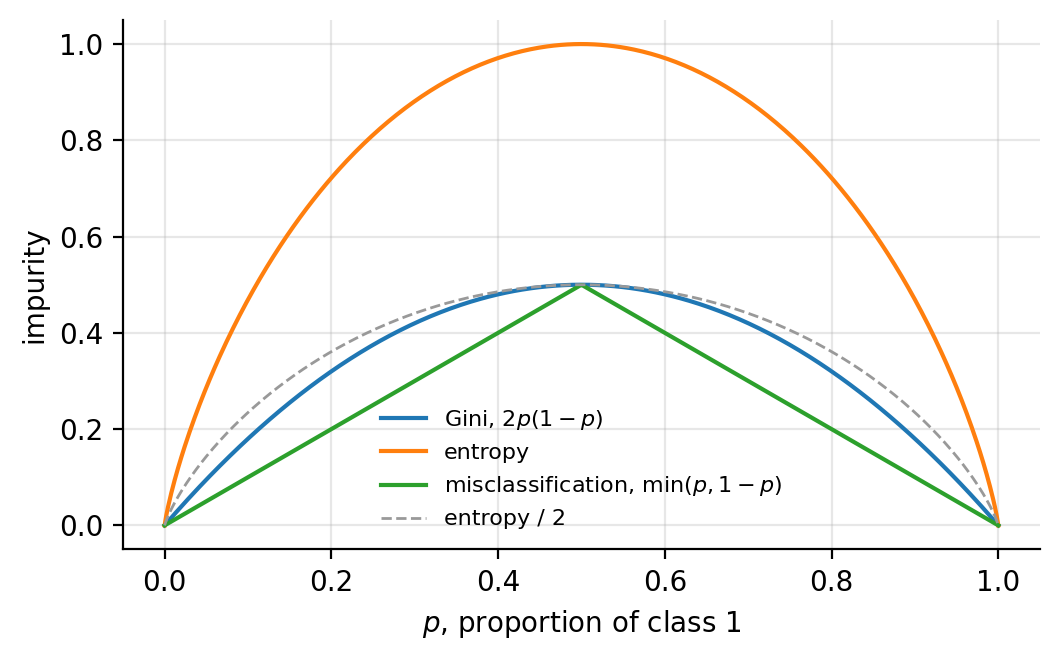
Figure 7.1: The three impurity measures of Eqs. (7.6)-(7.8) for a node with a fraction \(p\) of one class. The misclassification rate is piecewise linear, the Gini index and entropy strictly concave.
7.4. The CART algorithm#
Two algorithms dominate: CART (Classification And Regression Tree), used for
both tasks and implemented in scikit-learn, and ID3, based on
information gain and used for classification with categorical attributes.
CART for classification. CART splits the data set in two using a single feature \(k\) and a threshold \(t_k\), searching for the pair producing the purest subsets. The cost function it minimises is
where \(G_{\mathrm{left/right}}\) is the impurity of the corresponding subset and \(m_{\mathrm{left/right}}\) the number of instances in it. Having split the training set in two it splits each subset by the same logic, recursively, stopping when it reaches a maximum depth or can find no split reducing impurity. Further stopping conditions are controlled by the minimum number of samples required to split a node, the minimum number in a leaf, and the maximum number of leaves.
Equivalently one maximises the impurity decrease, or gain,
which is the form we shall implement. When the entropy is used in place of the Gini index, \(\Delta\) is called the information gain, and choosing splits by it is the ID3 algorithm: at each node one asks which attribute best separates the training examples, selects it, creates a descendant for each of its values, sorts the examples into the descendants, and repeats. The search is greedy and never backtracks.
CART for regression. The regression version is identical with the impurity replaced by the mean squared error,
where for a node
Note that Eq. (7.11) with these definitions is exactly Eq. (7.3) divided by \(m\), so the two formulations agree. Without regularisation – a depth limit or pruning – regression trees overfit just as classification trees do.
7.5. A worked example: computing the Gini index#
A classical example makes the arithmetic concrete. Based on meteorological attributes we wish to predict whether we go for a ride. The features are outlook (sunny, overcast, rain), temperature (hot, mild, cool), humidity (high, normal) and wind (weak, strong); the target is whether we ride (1) or do something else (0).
Day |
Outlook |
Temperature |
Humidity |
Wind |
Ride |
|---|---|---|---|---|---|
1 |
Sunny |
Hot |
High |
Weak |
0 |
2 |
Sunny |
Hot |
High |
Strong |
1 |
3 |
Overcast |
Hot |
High |
Weak |
1 |
4 |
Rain |
Mild |
High |
Weak |
1 |
5 |
Rain |
Cool |
Normal |
Weak |
1 |
6 |
Rain |
Cool |
Normal |
Strong |
0 |
7 |
Overcast |
Cool |
Normal |
Strong |
1 |
8 |
Sunny |
Mild |
High |
Weak |
0 |
9 |
Sunny |
Cool |
Normal |
Weak |
1 |
10 |
Rain |
Mild |
Normal |
Weak |
1 |
11 |
Sunny |
Mild |
Normal |
Strong |
1 |
12 |
Overcast |
Mild |
High |
Strong |
1 |
13 |
Overcast |
Hot |
Normal |
Weak |
1 |
14 |
Rain |
Mild |
High |
Strong |
0 |
Table 7.1: The ride data set: four categorical features and a binary target.
At the root there are \(10\) rides and \(4\) non-rides out of \(14\) days, so \(p_{m1}=10/14\) and \(p_{m0}=4/14\), giving by Eqs. (7.7) and (7.8)
Splitting on a categorical feature with several values, and scoring by the weighted average of Eq. (7.9), gives Table 7.2.
Feature |
Gini after split |
Entropy after split |
Information gain |
|---|---|---|---|
Outlook |
\(\mathbf{0.3429}\) |
\(\mathbf{0.6935}\) |
\(\mathbf{0.1696}\) |
Humidity |
\(0.3673\) |
\(0.7885\) |
\(0.0747\) |
Temperature |
\(0.4048\) |
\(0.8571\) |
\(0.0060\) |
Wind |
\(0.4048\) |
\(0.8571\) |
\(0.0060\) |
Table 7.2: Impurity after splitting the root of Table 7.1 on each feature. Outlook is chosen by both criteria. The information gain is \(S_{\mathrm{root}}\) minus the entropy after the split.
Both criteria select outlook as the root test, and for a visible reason: of its three values, overcast is perfectly pure – all four overcast days are rides – so that branch becomes a leaf immediately and needs no further splitting. Humidity is the next best, temperature and wind are nearly useless at the root. This is the ID3 algorithm performing its first step, and the whole tree is built by repeating the calculation within each impure branch.
7.6. Implementing a decision tree#
We now write CART from scratch. The implementation handles regression and classification, the three impurity measures, and – looking ahead to Sections Random forests and AdaBoost – both a random subset of features at each split and per-sample weights.
import numpy as np


def gini(y, classes):
    """Eq. (7.gini)."""
    p = np.array([np.mean(y == c) for c in classes])
    return 1.0 - np.sum(p**2)


def entropy(y, classes):
    """Eq. (7.entropy)."""
    p = np.array([np.mean(y == c) for c in classes])
    p = p[p > 0]
    return -np.sum(p * np.log2(p))


def mse_impurity(y):
    """Eq. (7.nodemse)."""
    return np.mean((y - y.mean())**2) if len(y) else 0.0


class Node:
    __slots__ = ("feature", "threshold", "left", "right", "value", "n")

    def __init__(self, value=None, n=0):
        self.feature = self.threshold = self.left = self.right = None
        self.value, self.n = value, n
The tree itself is a recursive search for the split maximising the impurity decrease (7.10).
class DecisionTree:
    """CART for regression and classification.

    task       : "classification" or "regression"
    criterion  : "gini" or "entropy" (classification only)
    max_features: if set, only a random subset of features is tried at each
                  split -- this is what turns bagging into a random forest.
    """

    def __init__(self, task="classification", criterion="gini", max_depth=None,
                 min_samples_split=2, min_samples_leaf=1, max_features=None,
                 rng=None):
        self.task, self.criterion = task, criterion
        self.max_depth = np.inf if max_depth is None else max_depth
        self.min_samples_split = min_samples_split
        self.min_samples_leaf = min_samples_leaf
        self.max_features = max_features
        self.rng = np.random.default_rng() if rng is None else rng

    def _impurity(self, y, w=None):
        if self.task == "regression":
            return mse_impurity(y)
        if w is None:
            return (gini(y, self.classes_) if self.criterion == "gini"
                    else entropy(y, self.classes_))
        p = np.array([w[y == c].sum() / w.sum() for c in self.classes_])
        if self.criterion == "gini":
            return 1.0 - np.sum(p**2)
        p = p[p > 0]
        return -np.sum(p * np.log2(p))

    def _leaf_value(self, y, w=None):
        if self.task == "regression":
            return y.mean()                       # the optimal constant
        counts = ([np.sum(y == c) for c in self.classes_] if w is None
                  else [w[y == c].sum() for c in self.classes_])
        return self.classes_[int(np.argmax(counts))]      # majority vote

    def _best_split(self, X, y, w):
        n, p = X.shape
        features = np.arange(p)
        if self.max_features is not None and self.max_features < p:
            features = self.rng.choice(p, self.max_features, replace=False)

        parent = self._impurity(y, w)
        W = w.sum() if w is not None else n
        best_gain, best_j, best_t = 0.0, None, None

        for j in features:
            xs = X[:, j]
            uniq = np.unique(xs)
            if len(uniq) < 2:
                continue
            for t in (uniq[:-1] + uniq[1:]) / 2.0:        # candidate midpoints
                mask = xs <= t
                nl, nr = mask.sum(), n - mask.sum()
                if nl < self.min_samples_leaf or nr < self.min_samples_leaf:
                    continue
                if w is None:
                    wl, wr = nl, nr
                else:
                    wl, wr = w[mask].sum(), w[~mask].sum()
                    if wl <= 0 or wr <= 0:
                        continue
                child = ((wl / W) * self._impurity(y[mask],
                                                   None if w is None else w[mask])
                         + (wr / W) * self._impurity(y[~mask],
                                                     None if w is None else w[~mask]))
                gain = parent - child                     # Eq. (7.gain)
                if gain > best_gain + 1e-12:
                    best_gain, best_j, best_t = gain, j, t
        return best_gain, best_j, best_t

    def _build(self, X, y, w, depth):
        node = Node(self._leaf_value(y, w), len(y))
        if (depth >= self.max_depth or len(y) < self.min_samples_split
                or len(np.unique(y)) == 1):
            return node
        gain, j, t = self._best_split(X, y, w)
        if j is None or gain <= 0:
            return node
        mask = X[:, j] <= t
        node.feature, node.threshold = j, t
        node.left = self._build(X[mask], y[mask],
                                None if w is None else w[mask], depth + 1)
        node.right = self._build(X[~mask], y[~mask],
                                 None if w is None else w[~mask], depth + 1)
        return node

    def fit(self, X, y, sample_weight=None):
        X, y = np.asarray(X, dtype=float), np.asarray(y)
        if self.task == "classification":
            self.classes_ = np.unique(y)
        self.root_ = self._build(X, y, sample_weight, 0)
        return self

    def predict(self, X):
        X = np.asarray(X, dtype=float)
        out = []
        for x in X:
            node = self.root_
            while node.feature is not None:               # walk to a leaf
                node = node.left if x[node.feature] <= node.threshold else node.right
            out.append(node.value)
        return np.array(out)
Checking it.
On the moons data of Section Kernels and non-linearity with \(400\) samples, our tree
and scikit-learn’s agree exactly at every depth we tried:
depth=1   ours train=0.8300 test=0.7500 | sklearn train=0.8300 test=0.7500
depth=3   ours train=0.9100 test=0.8100 | sklearn train=0.9100 test=0.8100
depth=5   ours train=0.9467 test=0.8900 | sklearn train=0.9467 test=0.9000
depth=inf ours train=1.0000 test=0.9000 | sklearn train=1.0000 test=0.8900
and on a regression problem the test mean squared errors agree to the last digit at depths \(2\) and \(4\) (\(6031.03\) and \(3097.39\)). The small disagreements at unlimited depth come from ties between equally good splits, broken differently by the two implementations.
The last row is the important one. The fully grown tree fits the training data perfectly and generalises worse than the tree of depth five: the classic overfitting signature of Section The bias-variance tradeoff, with the variance term growing without limit. Everything in the rest of this chapter is a way of controlling it.
Figure 7.2 shows the boundaries behind those numbers. At depth one the tree is a single threshold; at depth three it has the right gross shape; at depth five it is close to the truth. Grown without limit it develops narrow rectangular islands around individual training points – visibly fitting noise, and the geometric signature of the variance term. Note also that every boundary is a staircase of axis-aligned steps, since a tree can only ask questions of the form \(x_j\le t\).
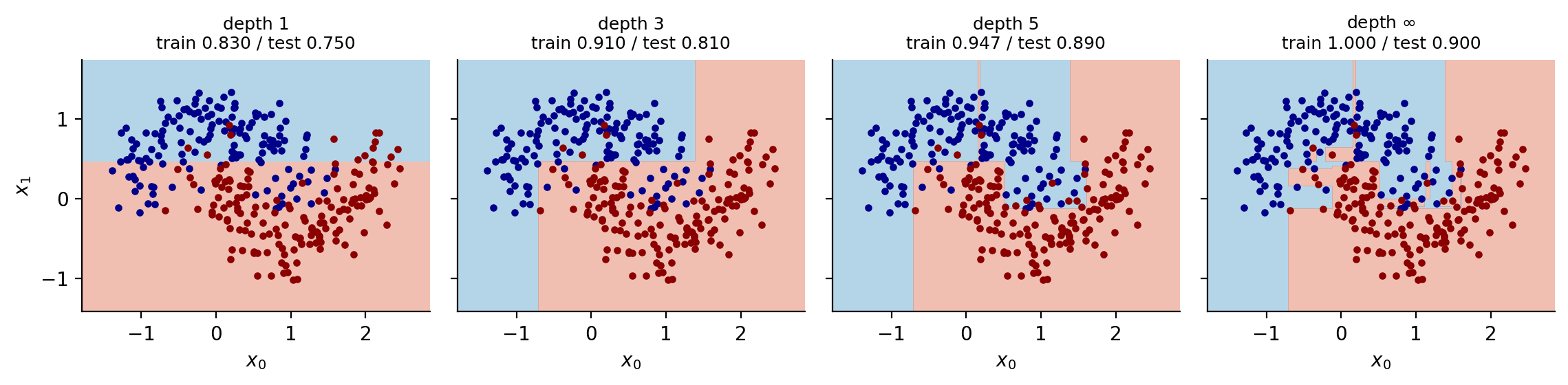
Figure 7.2: Decision boundaries of a single tree at four depths on the moons data. Growing the tree without limit produces isolated regions around individual points. All boundaries are unions of axis-aligned rectangles.
7.7. Strengths and weaknesses of trees#
In favour of trees: they are simple to understand and to interpret, and can be visualised; they require little data preparation, since no scaling or centring is needed – a monotone transformation of any feature leaves the tree unchanged, which no other method in this book can claim; the cost of prediction is logarithmic in the number of training points; they handle numerical and categorical data, and multiple outputs; and the model is a white box, so any prediction can be explained by the sequence of tests that produced it.
Against them: they readily overfit, producing trees that do not generalise, which is why pruning, depth limits and minimum leaf sizes are required; they are unstable, in that a small change in the data can produce a completely different tree, which is the high variance we have already seen; the greedy search gives no guarantee of the globally optimal tree, and finding that is NP-complete; they cannot express a diagonal decision boundary economically; and they are biased towards features with many possible split points, and towards the majority class in unbalanced problems.
The instability is the crucial defect and, paradoxically, the opportunity. An unstable, low-bias, high-variance predictor is exactly what averaging helps most, and the whole of the rest of this chapter follows from that observation.
7.8. Why averaging helps#
Before constructing any ensemble it is worth deriving how much averaging can gain, because the answer dictates the design of every method that follows.
Averaging independent predictors. Suppose we have \(B\) predictors \(\hat{f}_1,\dots,\hat{f}_B\), each unbiased for the target with variance \(\sigma^{2}\), and average them, \(\bar{f}=\tfrac1B\sum_b\hat{f}_b\). If they are independent then by the rules of Section Expectation values and moments
The bias is untouched and the variance falls as \(1/B\). Referred to the bias-variance decomposition (2.52), averaging attacks the variance term only – which is precisely why it is the right treatment for deep trees, whose bias is already small, and the wrong treatment for a model that is too rigid.
The catch: correlation. Predictors fitted to the same data set are not independent. If each pair has correlation \(\rho\), then expanding the variance of the average,
which simplifies to the central formula of this chapter,
Read it carefully. The second term vanishes as \(B\to\infty\): adding more predictors always helps, but with diminishing returns. The first term does not depend on \(B\) at all. However many trees we average, the variance cannot fall below \(\rho\sigma^{2}\).
Equation (7.16) is the design specification for everything that follows. To build a good ensemble we must make \(\sigma^{2}\) small (accurate members), make \(B\) large (many members) and – the part that is easy to overlook – make \(\rho\) small (diverse members). Bagging attacks \(\sigma^2/B\) by resampling; random forests exist because bagging alone leaves \(\rho\) too large; boosting takes an entirely different route, attacking the bias instead.
Figure 7.3 plots Eq. (7.16) for several correlations. For independent members the variance falls as \(1/B\) and can be made as small as we please. For correlated members it falls only until it reaches the floor \(\rho\sigma^{2}\), drawn as a dotted line, and thereafter additional trees are wasted effort. With \(\rho=0.8\) – not unusual for bagged trees sharing one dominant predictor – eighty per cent of the variance survives however many trees are grown. That floor is what the random forest is designed to lower.
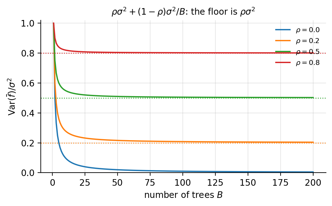
Figure 7.3: The variance of an average of \(B\) predictors, Eq. (7.16), for four values of the pairwise correlation \(\rho\). Dotted lines mark the floor \(\rho\sigma^{2}\), which no number of members can cross.
An aside on voting. For classification there is a complementary argument. Suppose \(B\) independent classifiers are each correct with probability \(p>1/2\) and we take a majority vote. The number correct is binomial, Eq. (2.11), and the probability that the majority is right tends to one as \(B\) grows – this is Condorcet’s jury theorem. A simple simulation makes it vivid: repeatedly tossing a coin with \(p=0.51\) and plotting the running fraction of heads, the curve wanders at first but settles above \(0.5\) with near certainty after a few thousand tosses. Weak but independent voters combine into a strong one. The italicised word is again independent, and again it is the assumption that reality violates.
7.9. Bagging#
Bootstrap aggregation, or bagging, applies Eq. (7.16) directly. We cannot draw \(B\) independent training sets – we have only one – so we manufacture them by the bootstrap of Section Resampling: the jackknife and the bootstrap: draw \(n\) observations with replacement, fit a tree, repeat \(B\) times, and average the predictions, or take a majority vote for classification.
Trees are grown deep and not pruned. This is deliberate: deep trees have low bias and high variance, averaging removes variance and leaves bias untouched, so we want the individual members to be as unbiased as possible and let the ensemble deal with the rest.
Out-of-bag estimation. Bagging comes with a free validation set. By the calculation in the exercises of Chapter 2, the probability that a given observation is not drawn in a particular bootstrap sample is
as \(n\) grows. About a third of the data is therefore omitted from each tree, and for each observation we may average the predictions of exactly those trees that did not see it. The resulting out-of-bag error is an almost unbiased estimate of the test error, obtained without any separate split or cross-validation. In our implementation the measured fraction is \(0.3683\) against the predicted \(0.3679\).
Interpretability, and what replaces it. Bagging improves accuracy at the expense of interpretability: a collection of hundreds of trees can no longer be drawn as one. What survives is a summary of variable importance. For regression one records the total reduction in mean squared error due to splits on each predictor, averaged over all \(B\) trees; for classification, the total reduction in the Gini index. A large value marks an important predictor. This is a genuine loss – the importance ranking is much less informative than a readable tree, and it is known to be biased towards high-cardinality features – but it is what remains.
7.10. Random forests#
Random forests improve on bagged trees by a small tweak that decorrelates them – that is, that attacks the \(\rho\sigma^{2}\) floor of Eq. (7.16).
As in bagging we build many trees on bootstrapped samples. But each time a split is considered, only a random sample of \(m\) of the \(p\) predictors is offered as a candidate, and the split must use one of those \(m\). A fresh sample is drawn at every split, and typically
for classification, with \(m\approx p/3\) often used for regression. At each split the algorithm is thus not even allowed to consider the majority of the available predictors.
Why this clever restriction works. Suppose one predictor is very strong and several others are moderately strong. In a bagged ensemble, most or all of the trees will place the strong predictor at the top split, so the trees will look very similar to one another and their predictions will be highly correlated. By Eq. (7.16), averaging many highly correlated quantities does not reduce variance much – the \(\rho\sigma^{2}\) term dominates. Forcing each split to ignore a random majority of the features means the strong predictor is unavailable in about \(1-m/p\) of the splits, so other predictors get their turn, and the trees genuinely differ.
There is a price. Restricting the candidate set means each individual tree is worse than it could be, so \(\sigma^{2}\) rises. The gain is a fall in \(\rho\). Random forests work because, for deep trees, the second effect outweighs the first – and \(m\) is the hyperparameter trading them off. Taking \(m=p\) recovers bagging exactly; taking \(m=1\) gives maximally decorrelated but very weak trees. Equation (7.18) is a rule of thumb, and \(m\) deserves cross-validation like any other hyperparameter.
class BaggingClassifier:
    """Bootstrap aggregation of unpruned trees, with out-of-bag scoring."""

    def __init__(self, n_estimators=100, max_depth=None, max_features=None,
                 rng=None):
        self.n_estimators, self.max_depth = n_estimators, max_depth
        self.max_features = max_features
        self.rng = np.random.default_rng(0) if rng is None else rng

    def fit(self, X, y):
        X, y = np.asarray(X, dtype=float), np.asarray(y)
        n = len(y)
        self.classes_ = np.unique(y)
        self.trees_, self.oob_ = [], []
        for _ in range(self.n_estimators):
            idx = self.rng.integers(0, n, n)            # bootstrap resample
            self.oob_.append(np.setdiff1d(np.arange(n), idx))
            tree = DecisionTree("classification", "gini", max_depth=self.max_depth,
                                max_features=self.max_features, rng=self.rng)
            self.trees_.append(tree.fit(X[idx], y[idx]))
        return self

    def predict(self, X):
        X = np.asarray(X, dtype=float)
        votes = np.stack([t.predict(X) for t in self.trees_])
        out = np.empty(X.shape[0], dtype=self.classes_.dtype)
        for i in range(X.shape[0]):                     # majority vote
            counts = [np.sum(votes[:, i] == c) for c in self.classes_]
            out[i] = self.classes_[int(np.argmax(counts))]
        return out

    def oob_score(self, X, y):
        """Eq. (7.oob): each point is scored by the trees that never saw it."""
        X, y = np.asarray(X, dtype=float), np.asarray(y)
        tally = np.zeros((len(y), len(self.classes_)))
        for tree, oob in zip(self.trees_, self.oob_):
            if len(oob) == 0:
                continue
            pred = tree.predict(X[oob])
            for k, c in enumerate(self.classes_):
                tally[oob[pred == c], k] += 1
        seen = tally.sum(axis=1) > 0
        vote = self.classes_[np.argmax(tally[seen], axis=1)]
        return np.mean(vote == y[seen])


class RandomForestClassifier(BaggingClassifier):
    """Bagging plus a random subset of m features at every split."""

    def __init__(self, n_estimators=100, max_depth=None, max_features="sqrt",
                 rng=None):
        super().__init__(n_estimators, max_depth, None, rng)
        self._mf = max_features

    def fit(self, X, y):
        p = np.asarray(X).shape[1]
        self.max_features = int(np.sqrt(p)) if self._mf == "sqrt" else self._mf
        return super().fit(X, y)          # Eq. (7.mtry)
On the moons data with \(500\) samples and noise \(0.30\), split into training and test sets, the from-scratch implementations give
single tree        test acc = 0.8560
bagging  (ours)    test acc = 0.8800   out-of-bag = 0.9013
bagging  (sklearn) test acc = 0.8960   out-of-bag = 0.9040
forest   (ours)    test acc = 0.8880   out-of-bag = 0.9040
forest   (sklearn) test acc = 0.8960   out-of-bag = 0.9067
Both ensembles improve substantially on the single tree, the forest edges out
plain bagging, and our figures track scikit-learn’s within the noise
of a \(125\)-point test set – for which, by Eq. (2.24), the
standard error of an accuracy near \(0.9\) is about \(0.027\), so none of these
differences is individually significant. The out-of-bag estimates, computed
on the \(375\) training points, are more reliable than the test figures and
tell the same story.
Machine learning connection
Random forests are close to the ideal off-the-shelf method for tabular data. They need no feature scaling, are insensitive to monotone transformations, handle mixed data types, cope with missing values, come with a free error estimate via Eq. (7.17), rarely overfit as \(B\) grows – adding trees only reduces the second term in Eq. (7.16), never the bias – and have essentially two hyperparameters, of which one is “as many trees as you can afford”. Their weaknesses follow from the same structure: they cannot extrapolate beyond the range of the training targets, since every prediction is an average of observed values; they produce axis-aligned boundaries; and they are large objects to store and slow to evaluate compared with a linear model.
7.11. Boosting: a bird’s eye view#
Bagging builds many strong learners in parallel and averages away their variance. Boosting does the opposite: it builds many weak learners sequentially, each correcting the errors of its predecessors, and reduces bias. A weak classifier is one performing only slightly better than random guessing – a tree of depth one, a stump, is the canonical example.
Boosting is a way of fitting an additive expansion in a set of elementary basis functions. Assume
where the \(\beta_m\) are expansion coefficients and \(b(x;\gamma_m)\) are simple functions characterised by parameters \(\gamma_m\). The reader has met this structure before. Taking \(b\) to be a sigmoid gives the model of Chapter 5, with \(t=\gamma_0+\gamma_1x\); taking \(b\) to be the coordinate functions gives linear regression, where \(\bm{f}=\bm{X}\bm{\theta}\) and the coefficients follow in closed form from Eq. (3.8). In boosting, \(b\) is a small decision tree and we must determine \(\beta_m\) and \(\gamma_m\) by minimising a cost function.
Minimising over all \(M\) terms jointly is intractable. The essential idea is forward stagewise fitting: having built \(f_{m-1}\), we add one term,
choosing \((\beta_m,\gamma_m)\) to minimise the cost given \(f_{m-1}\), which is never revisited. Everything in the rest of this chapter is a specialisation of Eq. (7.20) to a particular loss.
7.12. AdaBoost#
Take binary classification with \(y_i\in\{-1,1\}\) and a classifier \(G(x)\) returning one of the two values. The training error rate is
We shall produce a sequence of weak classifiers \(G_m(x)\) applied to repeatedly modified versions of the data, and combine them as
The exponential loss. The choice of loss which makes the algebra collapse – and which historically produced AdaBoost – is the exponential loss,
Note that the argument \(y_if(x_i)\) is the margin met in Section The primal view: the hinge loss: positive when correct, and the loss decays exponentially with it. Inserting the stagewise form (7.20),
where \(w_i^m\) depends on neither \(\beta\) nor \(G\) and therefore acts as a weight attached to observation \(i\). This is the key structural fact: minimising the exponential loss stagewise is the same as fitting a weighted classifier, with weights that grow for the observations previous rounds got wrong.
Solving for \(G\) and \(\beta\). Since \(y_iG(x_i)=+1\) when correct and \(-1\) when not, split the sum,
For any \(\beta>0\) the first factor is positive, so \(C\) is minimised over \(G\) by minimising the weighted error rate – the weak learner is simply fitted to the weighted data. Defining
and differentiating Eq. (7.25) with respect to \(\beta\) gives \(-e^{-\beta}(1-\overline{\mathrm{err}}_m)+e^{\beta}\overline{\mathrm{err}}_m=0\), whence
Updating \(f_m=f_{m-1}+\beta_mG_m\) propagates into the weights through Eq. (7.24),
and since \(-y_iG_m(x_i)=2I(y_i\ne G_m(x_i))-1\), this equals \(w_i^m e^{-\beta_m}\exp\left(\alpha_mI(y_i\ne G_m(x_i))\right)\) with
The common factor \(e^{-\beta_m}\) is the same for every \(i\) and disappears on renormalising the weights, which is why the algorithm is usually stated with \(\alpha_m\) rather than \(\beta_m\).
The algorithm.
Initialise \(w_i=1/n\) for \(i=0,\dots,n-1\), so that \(\sum_iw_i=1\).
For \(m=1,\dots,M\):
fit the weak classifier \(G_m\) to the training data using weights \(w_i\);
compute the weighted error (7.26);
set \(\alpha_m\) by Eq. (7.29);
update \(w_i\leftarrow w_i\exp\left(\alpha_mI(y_i\ne G_m(x_i))\right)\) and renormalise.
Output the combined classifier (7.22).
Observations misclassified at round \(m\) receive a larger weight at round \(m+1\), so each new learner is forced to concentrate on the cases its predecessors found difficult. Note that \(\alpha_m>0\) exactly when \(\overline{\mathrm{err}}_m<1/2\), so a learner better than chance gets a positive vote and one worse than chance gets a negative one – it is used with its predictions inverted, which is correct rather than perverse.
class AdaBoost:
    """Discrete AdaBoost with decision stumps; labels must be -1 and +1."""

    def __init__(self, n_estimators=50, max_depth=1, rng=None):
        self.n_estimators, self.max_depth = n_estimators, max_depth
        self.rng = np.random.default_rng(0) if rng is None else rng

    def fit(self, X, y):
        X, y = np.asarray(X, dtype=float), np.asarray(y, dtype=float)
        n = len(y)
        w = np.full(n, 1.0 / n)                     # step 1
        self.trees_, self.alphas_ = [], []

        for _ in range(self.n_estimators):
            tree = DecisionTree("classification", "gini",
                                max_depth=self.max_depth, rng=self.rng)
            tree.fit(X, y, sample_weight=w)         # weighted weak learner
            miss = (tree.predict(X) != y).astype(float)

            err = np.sum(w * miss) / np.sum(w)      # Eq. (7.weightederr)
            err = min(max(err, 1e-10), 1 - 1e-10)
            alpha = np.log((1 - err) / err)         # Eq. (7.alpha)

            w = w * np.exp(alpha * miss)            # Eq. (7.weightupdate)
            w /= w.sum()

            self.trees_.append(tree)
            self.alphas_.append(alpha)
            if err <= 1e-10:                        # a perfect learner: stop
                break
        return self

    def decision_function(self, X):
        return np.sum([a * t.predict(X)
                       for a, t in zip(self.alphas_, self.trees_)], axis=0)

    def predict(self, X):
        return np.sign(self.decision_function(X))   # Eq. (7.adacombine)
On the moons data our implementation reaches a test accuracy of \(0.9040\) with
\(200\) stumps, exactly matching scikit-learn’s
AdaBoostClassifier with the same settings. Tracking the error as
stumps accumulate shows the characteristic behaviour:
M=  1: train err=0.1813  test err=0.1760
M=  5: train err=0.1147  test err=0.1040
M= 20: train err=0.0720  test err=0.0960
M= 50: train err=0.0720  test err=0.0960
M=100: train err=0.0693  test err=0.0880
M=200: train err=0.0480  test err=0.0960
A single stump is a poor classifier, and a few hundred of them together are a good one – the promise of boosting, delivered. Note also that the training error keeps falling after the test error has stopped improving, so \(M\) is a hyperparameter to be cross-validated and not increased indefinitely.
Machine learning connection
Why the exponential loss? It is not merely convenient. One can show that the function minimising the population exponential loss is
one half the log-odds – exactly the quantity logistic regression models in Eq. (5.10). AdaBoost is therefore estimating the same object as Chapter 5, by a completely different route, and \(\sigma(2f)\) recovers a probability. The difference lies in the tails: the exponential loss grows as \(e^{-yf}\) for badly misclassified points whereas the logistic loss grows only linearly, so AdaBoost is markedly more sensitive to mislabelled data and to outliers. This is the same comparison made for the hinge loss in Section The primal view: the hinge loss, and it is why gradient boosting with a logistic loss – the subject of the next section – has largely displaced AdaBoost in practice.
7.13. Gradient boosting#
AdaBoost is tied to one loss. Gradient boosting generalises it to any differentiable loss, and the generalisation comes from an idea we have already developed at length: gradient descent, now performed in function space.
Functional gradient descent. Write the cost as a sum over observations, \(C(\bm{y},\bm{f})=\sum_{i}L\left(y_i,f(x_i)\right)\), and regard the \(n\) numbers \(f(x_i)\) as the parameters to be optimised. Gradient descent, in the sense of Eq. (4.10), would compute
and update \(f_m=f_{m-1}-\rho_mg_m\). For the squared error \(L=(y_i-f(x_i))^{2}\) the gradient is \(g_m(x_i)=-2\left(y_i-f_{m-1}(x_i)\right)\) – proportional to the residual.
This literal steepest descent is not useful. It optimises \(f\) at the \(n\) training points only, producing a table of values rather than a function, so it cannot generalise to a new \(x\). The remedy is the whole idea of gradient boosting: fit a weak learner to approximate the negative gradient. The learner interpolates the gradient signal to the rest of the space, and adding it moves \(f\) downhill everywhere rather than at \(n\) points.
The algorithm.
Initialise \(f_0(x)\), usually the constant minimising the loss.
For \(m=1,\dots,M\):
compute the negative gradient, or pseudo-residual, \(u_{im}=-\left[\partial L(y_i,f(x_i))/\partial f(x_i)\right]_{f=f_{m-1}}\);
fit a base learner \(h_m\) to the pairs \((x_i,u_{im})\) – a regression tree, whatever the original task;
update \(f_m(x)=f_{m-1}(x)+\nu\,h_m(x)\).
Return \(f_M(x)=f_0(x)+\nu\sum_{m=1}^{M}h_m(x)\).
The factor \(\nu\in(0,1]\) is the learning rate or shrinkage, playing exactly the role it played in Chapter 4: small steps, many of them. Values around \(0.1\) are typical, and \(\nu\) and \(M\) trade off directly against each other – halving \(\nu\) roughly doubles the \(M\) required.
Squared error: boosting on residuals. For \(L=\tfrac12(y-f)^{2}\) the pseudo-residual is
the ordinary residual. Gradient boosting with squared error is therefore disarmingly simple: fit a tree to the data, compute what is left over, fit a tree to that, and repeat. Each tree corrects its predecessors’ mistakes.
Logistic loss: boosting for classification. For binary classification with \(y\in\{0,1\}\) we model the log-odds, as in Eq. (5.10), setting \(p=\sigma(f)\) and taking \(L\) to be the cross entropy (5.13). Then
using \(d\sigma/dt=\sigma(1-\sigma)\) from Eq. (5.5) and the cancellation noted in the notebox of Section Maximum likelihood and the cross-entropy. Once again the pseudo-residual is target minus prediction, now on the probability scale, and once again we fit a regression tree to it. The natural initialisation is the constant log-odds of the training set, \(f_0=\log\left(\bar{y}/(1-\bar{y})\right)\).
class GradientBoostingRegressor:
    """Gradient boosting with the squared-error loss, Eq. (7.gbresidual)."""

    def __init__(self, n_estimators=100, learning_rate=0.1, max_depth=3,
                 rng=None):
        self.n_estimators, self.lr = n_estimators, learning_rate
        self.max_depth = max_depth
        self.rng = np.random.default_rng(0) if rng is None else rng

    def fit(self, X, y):
        X, y = np.asarray(X, dtype=float), np.asarray(y, dtype=float)
        self.f0_ = y.mean()                       # the optimal constant
        f = np.full(len(y), self.f0_)
        self.trees_ = []
        for _ in range(self.n_estimators):
            residual = y - f                      # negative gradient
            tree = DecisionTree("regression", max_depth=self.max_depth,
                                rng=self.rng).fit(X, residual)
            f = f + self.lr * tree.predict(X)     # shrunken update
            self.trees_.append(tree)
        return self

    def predict(self, X):
        X = np.asarray(X, dtype=float)
        f = np.full(X.shape[0], self.f0_)
        for tree in self.trees_:
            f = f + self.lr * tree.predict(X)
        return f


class GradientBoostingClassifier:
    """Binary gradient boosting on the logistic loss, Eq. (7.gblogistic).

    Labels must be 0 and 1.  The model is additive in the log-odds.
    """

    def __init__(self, n_estimators=100, learning_rate=0.1, max_depth=3,
                 rng=None):
        self.n_estimators, self.lr = n_estimators, learning_rate
        self.max_depth = max_depth
        self.rng = np.random.default_rng(0) if rng is None else rng

    def fit(self, X, y):
        X, y = np.asarray(X, dtype=float), np.asarray(y, dtype=float)
        pbar = np.clip(y.mean(), 1e-6, 1 - 1e-6)
        self.f0_ = np.log(pbar / (1 - pbar))      # constant log-odds
        f = np.full(len(y), self.f0_)
        self.trees_ = []
        for _ in range(self.n_estimators):
            p = 1.0 / (1.0 + np.exp(-f))
            residual = y - p                      # Eq. (7.gblogistic)
            tree = DecisionTree("regression", max_depth=self.max_depth,
                                rng=self.rng).fit(X, residual)
            f = f + self.lr * tree.predict(X)
            self.trees_.append(tree)
        return self

    def decision_function(self, X):
        X = np.asarray(X, dtype=float)
        f = np.full(X.shape[0], self.f0_)
        for tree in self.trees_:
            f = f + self.lr * tree.predict(X)
        return f

    def predict_proba(self, X):
        p = 1.0 / (1.0 + np.exp(-self.decision_function(X)))
        return np.column_stack([1 - p, p])

    def predict(self, X):
        return (self.decision_function(X) > 0).astype(int)
Both are checked against scikit-learn. On the moons data with \(200\)
trees of depth two and \(\nu=0.1\) our classifier reaches a test accuracy of
\(0.9120\) against \(0.8960\); on a five-feature regression problem with the same
settings our test mean squared error is \(932.86\) against \(934.03\). The
agreement is as close as the tie-breaking in the underlying trees permits.
Machine learning connection
Gradient boosting is where several threads of this book meet. The optimisation is that of Chapter 4, moved from parameter space to function space, with \(\nu\) the learning rate and \(M\) the number of steps – so that stopping early is exactly the early stopping of Section Learning rate schedules and stopping, and is the main regularisation available. The loss is chosen by the argument of Section Deriving least squares from a probability distribution: squared error for Gaussian noise, logistic for Bernoulli targets, and any other differentiable loss one can write down, including the quantile and Huber losses for robust regression – Section Boosting any loss: automatic differentiation does exactly that, with the derivatives supplied by automatic differentiation. The base learner is the tree of Section Implementing a decision tree. And the contrast with bagging is instructive: bagging averages independent deep trees to remove variance, boosting sums dependent shallow trees to remove bias. Because boosting reduces bias by construction, it can overfit as \(M\) grows, which random forests essentially cannot – so the two families need opposite habits of mind about how many trees to use.
Figure 7.4 shows both families in action. On the left, both bagging and the random forest improve rapidly on the single tree and then flatten, exactly as Eq. (7.16) requires, with the forest holding a small advantage from its lower \(\rho\). On the right, AdaBoost’s training error falls steadily towards zero as stumps accumulate while the test error flattens after a few dozen: boosting reduces bias without limit and will eventually overfit, which is precisely the behaviour bagging does not show.
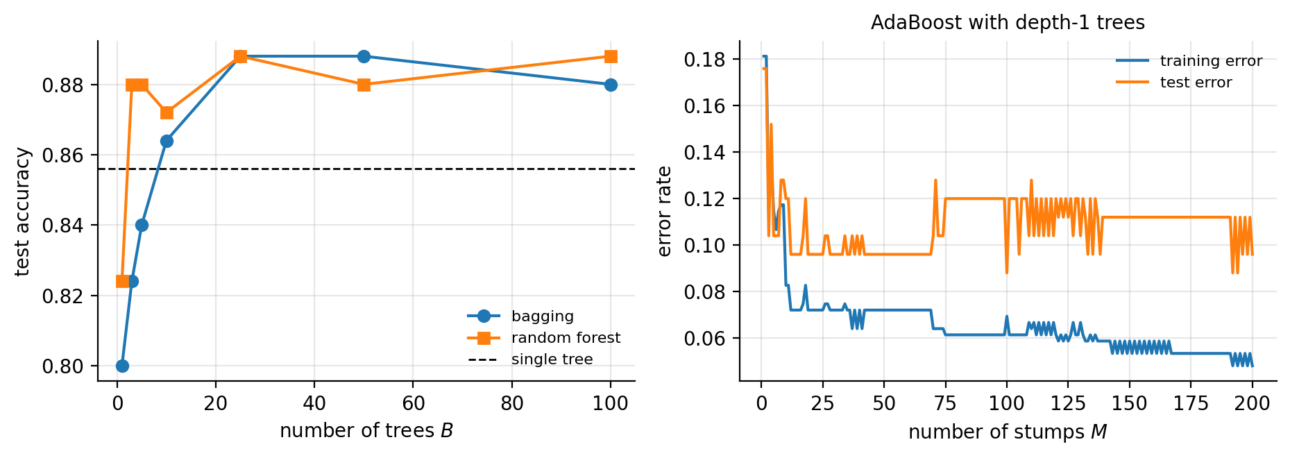
Figure 7.4: Left: test accuracy of bagging and of a random forest against the number of trees, with the single tree marked. Right: AdaBoost training and test error against the number of stumps. The two panels contrast variance reduction with bias reduction.
7.14. XGBoost: extreme gradient boosting#
XGBoost is the best known of the modern boosting libraries, and it differs from Section Gradient boosting in two mathematical respects worth deriving, even though here we shall use the library rather than write our own.
A second-order objective. Ordinary gradient boosting uses only the first derivative of the loss. XGBoost expands the loss to second order around the current prediction. Writing \(g_i=\partial L(y_i,f)/\partial f\) and \(h_i=\partial^{2}L(y_i,f)/\partial f^{2}\) evaluated at \(f_{m-1}(x_i)\), and letting the new tree contribute \(f_m(x_i)\), a Taylor expansion of the kind used in Section Newton’s method gives
where the constant \(L(y_i,f_{m-1})\) has been dropped and \(\Omega\) is an explicit complexity penalty on the tree,
with \(T\) the number of leaves and \(w_j\) the value in leaf \(j\). This is Ridge-style regularisation, Eq. (3.43), applied to the leaf weights, plus a per-leaf cost \(\gamma\) which is the cost-complexity penalty of Eq. (7.4) built into the objective rather than applied afterwards.
The closed-form leaf weight. A tree assigns a single value \(w_j\) to every point in leaf \(j\), so writing \(I_j\) for the set of observations landing there, Eq. (7.33) becomes
This is a sum of independent one-dimensional quadratics, so each is minimised exactly, by the argument of Section Four worked examples,
The second expression is a score for a tree structure – the smaller the better – and it gives a principled splitting criterion. Splitting a leaf into left and right parts changes the score by
Equation (7.37) replaces the Gini or MSE criterion of Section The CART algorithm: it is derived from the loss rather than chosen, it incorporates the regularisation, and the subtraction of \(\gamma\) means a split whose gain does not exceed \(\gamma\) is simply not made – pruning becomes part of growing.
Beyond the mathematics, XGBoost owes its reputation to engineering: sparsity awareness with a default direction for missing values, an approximate split-finding algorithm using quantile sketches, cache-aware access patterns, and parallel and out-of-core computation. These make it fast rather than different, and they are the reason we use the library here.
import xgboost as xgb
from sklearn.model_selection import train_test_split
from sklearn.metrics import accuracy_score, mean_squared_error

X_train, X_test, y_train, y_test = train_test_split(X, y, random_state=42)

# Classification. reg_lambda is the lambda of Eq. (7.xgbpenalty) and
# gamma the per-leaf cost of Eq. (7.xgbgain).
clf = xgb.XGBClassifier(n_estimators=200, learning_rate=0.1, max_depth=3,
                        reg_lambda=1.0, gamma=0.0, subsample=0.8,
                        colsample_bytree=0.8, eval_metric="logloss")
clf.fit(X_train, y_train)
print("accuracy:", accuracy_score(y_test, clf.predict(X_test)))

# Regression, with early stopping on a validation set
reg = xgb.XGBRegressor(n_estimators=1000, learning_rate=0.05, max_depth=4,
                       early_stopping_rounds=20)
reg.fit(X_train, y_train, eval_set=[(X_test, y_test)], verbose=False)
print("best iteration:", reg.best_iteration)
Note subsample and colsample_bytree: these apply the
bootstrap of Section Bagging and the feature subsampling of
Section Random forests within boosting, so that the modern
gradient boosting machine borrows from the bagging family as well. The
distinction drawn in this chapter between the two approaches is real
mathematically and blurred in practice.
7.15. Boosting any loss: automatic differentiation#
Sections Gradient boosting and XGBoost: extreme gradient boosting both needed
derivatives of the loss – the pseudo-residual \(u_{im}=-g_i\) of
Eq. (7.30), and the pair \(g_i,h_i\) of
Eq. (7.33) – and both times we derived them by hand,
Eqs. (7.31) and (7.32), for the two
losses we happened to want. That is exactly the situation
Section Automatic differentiation was written for, and here the payoff is
unusually clean. A tree is not differentiable: its split decisions are
discrete and automatic differentiation has nothing to say about them. But a
boosted tree never looks at the targets directly. It looks only at \(g_i\) and
\(h_i\), and those are derivatives of a one-line function. Everything that
depends on the loss can therefore be handed to JAX, and everything that
depends on the tree stays exactly as it was. The result is a boosting
machine in which the loss is an argument, as in
Section Other loss functions, and automatic differentiation, and which reproduces XGBoost to
single precision.
The losses and their derivatives.
Each loss is written pointwise, as a function of one target \(y\) and one
prediction \(f\); vmap maps it over the data, and grad applied
once and twice supplies \(g_i\) and \(h_i\).
import numpy as np
import jax
jax.config.update("jax_enable_x64", True)
import jax.numpy as jnp
from jax import grad, vmap, jit
from jax.nn import softplus, sigmoid

# Pointwise losses L(y, f).  f is the additive model: the value itself for
# regression, the log-odds for classification, the log-rate for counts.
def squared(y, f):
    return 0.5 * (y - f)**2                                # Eq. (7.gbresidual)

def logistic(y, f):
    return softplus(f) - y * f                             # cross entropy, f = log-odds

def huber(y, f, delta=1.0):
    r = jnp.abs(y - f)
    return jnp.where(r <= delta, 0.5 * r**2, delta * (r - 0.5 * delta))

def quantile(y, f, tau=0.9):
    r = y - f
    return jnp.maximum(tau * r, (tau - 1.0) * r)           # pinball loss

def poisson(y, f):
    return jnp.exp(f) - y * f                              # counts, f = log(rate)

def derivatives(loss):
    """g_i = dL/df and h_i = d^2L/df^2 at every data point, from JAX."""
    g = jit(vmap(grad(loss, argnums=1)))
    h = jit(vmap(grad(grad(loss, argnums=1), argnums=1)))
    return g, h
Two of these deserve a remark. The Huber loss is quadratic for \(|y-f|\le\delta\) and linear beyond, so its gradient is the residual clipped to \(\pm\delta\): a gross outlier pulls with bounded force. The quantile or pinball loss has gradient \(-\tau\) for \(y>f\) and \(1-\tau\) for \(y<f\), so its minimising constant is the \(\tau\)-quantile of the targets, and its second derivative is zero everywhere: JAX returns exactly that, and the second-order method below will therefore refuse it, which is correct – Newton’s method has nothing to work with on a piecewise-linear loss, and it must be boosted to first order.
The tree that sees only derivatives. The tree of Section XGBoost: extreme gradient boosting is grown on the vectors \(\bm{g}\) and \(\bm{h}\) alone: its split criterion is the gain (7.37) and its leaf values are Eq. (7.36). It is a smaller object than the CART of Section Implementing a decision tree, because there is no impurity to choose and no leaf value to vote on, and it contains ordinary gradient boosting as a special case. Set every \(h_i=1\) and \(\lambda=0\); then \(H_L=n_L\), \(H_R=n_R\), and the gain becomes
with \(u_i=-g_i\) the pseudo-residual: one half the reduction in the residual sum of squares obtained by splitting, which is precisely the criterion (7.12) of a least-squares regression tree fitted to \(u\), and the leaf value \(-G_j/H_j=\bar u_j\) is the leaf mean. (The identity is the analysis-of-variance decomposition of Eq. (3.20) applied within a node.) So a single tree builder serves both algorithms of this chapter: fed \(h\equiv1\) it is Friedman’s base learner, fed the true second derivatives it is XGBoost’s.
class Node:
    __slots__ = ("feature", "threshold", "left", "right", "value")
    def __init__(self, value):
        self.feature = self.threshold = self.left = self.right = None
        self.value = value

class GradientTree:
    """A regression tree grown on the derivatives g_i, h_i of the loss.

    Split criterion: the gain of Eq. (7.xgbgain); leaf value: Eq. (7.xgbweight).
    With h_i = 1 and lmbda = 0 it is a least-squares tree fitted to the
    pseudo-residual -g_i, Eq. (7.gainmse); with the true h_i it is XGBoost's tree.
    """
    def __init__(self, max_depth=3, lmbda=1.0, gamma=0.0, min_child_weight=1.0):
        self.max_depth, self.lmbda, self.gamma = max_depth, lmbda, gamma
        self.min_child_weight = min_child_weight

    def _build(self, X, g, h, depth):
        G, H = g.sum(), h.sum()
        node = Node(-G / (H + self.lmbda))                    # Eq. (7.xgbweight)
        if depth >= self.max_depth or len(g) < 2:
            return node
        best_gain, best_j, best_t = 0.0, None, None
        parent = G**2 / (H + self.lmbda)
        for j in range(X.shape[1]):
            order = np.argsort(X[:, j])
            xs, gs, hs = X[order, j], g[order], h[order]
            GL, HL = np.cumsum(gs)[:-1], np.cumsum(hs)[:-1]   # sums left of each split
            GR, HR = G - GL, H - HL
            gain = 0.5 * (GL**2 / (HL + self.lmbda)
                          + GR**2 / (HR + self.lmbda) - parent) - self.gamma
            valid = ((xs[:-1] < xs[1:]) & (HL >= self.min_child_weight)
                     & (HR >= self.min_child_weight))
            gain = np.where(valid, gain, -np.inf)              # Eq. (7.xgbgain)
            k = int(np.argmax(gain))
            if gain[k] > best_gain:
                best_gain, best_j, best_t = gain[k], j, 0.5 * (xs[k] + xs[k + 1])
        if best_j is None:
            return node
        mask = X[:, best_j] <= best_t
        node.feature, node.threshold = best_j, best_t
        node.left = self._build(X[mask], g[mask], h[mask], depth + 1)
        node.right = self._build(X[~mask], g[~mask], h[~mask], depth + 1)
        return node

    def fit(self, X, g, h):
        self.root_ = self._build(np.asarray(X, float), np.asarray(g), np.asarray(h), 0)
        return self

    def predict(self, X):
        out = []
        for x in np.asarray(X, float):
            node = self.root_
            while node.feature is not None:
                node = node.left if x[node.feature] <= node.threshold else node.right
            out.append(node.value)
        return np.array(out)
Note the cumulative sums: for each feature the candidate splits are scanned in sorted order and \(G_L,H_L\) are accumulated once, so the search costs \(\bigO(np\log n)\) per tree rather than the \(\bigO(n^{2}p)\) of the naive loop in Section Implementing a decision tree. This is the “exact” split finder of the libraries; their “histogram” method bins the features first and is faster still.
The boosting loop. What remains is the loop of Section Gradient boosting, with two additions. The initial constant \(f_0\) is the minimiser of \(\sum_iL(y_i,c)\), which for a convex loss is where the monotone function \(c\mapsto\sum_ig_i(c)\) crosses zero, so a bisection finds it for every loss at once – the mean for the squared error, the log-odds of the class frequency for the logistic loss, the \(\tau\)-quantile for the pinball loss – without a case distinction. And a switch selects first- or second-order boosting by deciding what the tree is fed as \(\bm{h}\).
class Boosting:
    """Gradient boosting for any pointwise loss, with all derivatives from JAX.

    order=1: Friedman's gradient boosting -- the tree fits the negative
             gradient by least squares (h_i = 1, lmbda = 0), Section 7.gradientboosting;
    order=2: Newton boosting as in XGBoost -- the tree is grown on g_i, h_i
             with the regularised gain and leaf weights of Section 7.xgboost.
    """
    def __init__(self, loss, order=2, n_estimators=100, learning_rate=0.1,
                 max_depth=3, lmbda=1.0, gamma=0.0, min_child_weight=1.0, f0=None):
        self.loss, self.order = loss, order
        self.g, self.h = derivatives(loss)
        self.n_estimators, self.lr, self.f0 = n_estimators, learning_rate, f0
        self.tree_kw = dict(max_depth=max_depth, gamma=gamma,
                            lmbda=lmbda if order == 2 else 0.0,
                            min_child_weight=min_child_weight if order == 2 else 0.0)

    def _constant(self, y):
        """The constant minimising sum_i L(y_i, c): bisection on the monotone sum of g."""
        lo, hi = min(float(y.min()), -50.0) - 1.0, max(float(y.max()), 50.0) + 1.0
        for _ in range(100):
            mid = 0.5 * (lo + hi)
            if float(jnp.sum(self.g(y, jnp.full(len(y), mid)))) > 0:
                hi = mid
            else:
                lo = mid
        return 0.5 * (lo + hi)

    def fit(self, X, y):
        y = jnp.asarray(y, dtype=float)
        self.f0_ = self._constant(y) if self.f0 is None else self.f0
        f = jnp.full(len(y), self.f0_)
        self.trees_ = []
        for _ in range(self.n_estimators):
            g = self.g(y, f)                                    # pseudo-residual is -g
            h = self.h(y, f) if self.order == 2 else jnp.ones_like(g)
            tree = GradientTree(**self.tree_kw).fit(X, g, h)
            f = f + self.lr * jnp.asarray(tree.predict(X))     # shrunken update
            self.trees_.append(tree)
        return self

    def decision_function(self, X):
        f = np.full(np.asarray(X).shape[0], self.f0_)
        for tree in self.trees_:
            f = f + self.lr * tree.predict(X)
        return f
Checking it against the derivations and against the library.
First the derivatives: for the logistic loss JAX must return
\(g_i=p_i-y_i\) and \(h_i=p_i(1-p_i)\), Eq. (7.32) and the
weights of Eq. (5.18). Then the whole machine, second order,
against XGBoost with the same hyperparameters on the moons data of
Section Implementing a decision tree; and finally first order, against the numbers of
Section Gradient boosting.
from sklearn.datasets import make_moons, make_regression
from sklearn.model_selection import train_test_split
import xgboost as xgb

g, h = derivatives(logistic)
y0, f0 = jnp.array([0., 1., 1., 0.]), jnp.array([-1., 0.3, 2., 0.1])
print("g - (p - y):", float(jnp.max(jnp.abs(g(y0, f0) - (sigmoid(f0) - y0)))))
print("h - p(1-p): ", float(jnp.max(jnp.abs(h(y0, f0) - sigmoid(f0) * (1 - sigmoid(f0))))))

X, y = make_moons(n_samples=500, noise=0.3, random_state=42)
X_train, X_test, y_train, y_test = train_test_split(X, y, random_state=42)

ours = Boosting(logistic, order=2, n_estimators=100, learning_rate=0.1,
                max_depth=3, lmbda=1.0, f0=0.0).fit(X_train, y_train)
lib = xgb.XGBClassifier(n_estimators=100, learning_rate=0.1, max_depth=3,
                        reg_lambda=1.0, gamma=0.0, min_child_weight=1.0,
                        base_score=0.5, tree_method="exact").fit(X_train, y_train)
p_ours = 1.0 / (1.0 + np.exp(-ours.decision_function(X_test)))
p_lib = lib.predict_proba(X_test)[:, 1]
print("max |p_ours - p_xgboost| =", np.max(np.abs(p_ours - p_lib)))
print("test accuracy: ours", np.mean((p_ours > 0.5) == y_test),
      " xgboost", np.mean((p_lib > 0.5) == y_test))

first = Boosting(logistic, order=1, n_estimators=200, learning_rate=0.1,
                 max_depth=2).fit(X_train, y_train)
print("first-order, 200 trees of depth 2: test accuracy",
      np.mean((first.decision_function(X_test) > 0) == y_test))
g - (p - y): 1.1102230246251565e-16
h - p(1-p):  2.7755575615628914e-17
max |p_ours - p_xgboost| = 1.1242810449285656e-07
test accuracy: ours 0.896  xgboost 0.896
first-order, 200 trees of depth 2: test accuracy 0.912
The derivatives are exact. The second-order machine agrees with
XGBoost to \(10^{-7}\) in every predicted probability, which is the
single precision the library computes in: fifty lines of Python and the
equations of Section XGBoost: extreme gradient boosting are the algorithm, and the
library adds speed rather than mathematics. And the first-order machine
reproduces the \(0.912\) of the hand-written
GradientBoostingClassifier of Section Gradient boosting,
as Eq. (7.38) says it must.
Changing the loss. Now the point of the exercise. A regression problem is given twenty gross outliers, and boosted under the squared error and under the Huber loss; then the same data are boosted under the pinball loss for three quantiles. Not one line of the machinery changes.
rng = np.random.default_rng(1)
Xr, yr = make_regression(n_samples=400, n_features=5, noise=10.0, random_state=1)
Xr_train, Xr_test, yr_train, yr_test = train_test_split(Xr, yr, random_state=1)
yr_dirty = yr_train.copy()
bad = rng.choice(len(yr_train), 20, replace=False)
yr_dirty[bad] += rng.choice([-1.0, 1.0], 20) * 500.0            # twenty gross outliers

for name, loss in [("squared error", squared),
                   ("Huber, delta=20", lambda y, f: huber(y, f, 20.0))]:
    for label, target in [("clean   ", yr_train), ("outliers", yr_dirty)]:
        model = Boosting(loss, order=1, n_estimators=300, learning_rate=0.1,
                         max_depth=3).fit(Xr_train, target)
        mse = np.mean((model.decision_function(Xr_test) - yr_test)**2)
        print(f"{name:16s} trained on {label} data: test MSE = {mse:7.1f}")

for tau in [0.1, 0.5, 0.9]:
    model = Boosting(lambda y, f: quantile(y, f, tau), order=1, n_estimators=300,
                     learning_rate=0.1, max_depth=3).fit(Xr_train, yr_train)
    below = np.mean(yr_test < model.decision_function(Xr_test))
    print(f"quantile loss, tau = {tau}: fraction of test targets below = {below:.3f}")
squared error    trained on clean    data: test MSE =   826.0
squared error    trained on outliers data: test MSE =  4237.1
Huber, delta=20  trained on clean    data: test MSE =  1012.8
Huber, delta=20  trained on outliers data: test MSE =  1053.5
quantile loss, tau = 0.1: fraction of test targets below = 0.120
quantile loss, tau = 0.5: fraction of test targets below = 0.530
quantile loss, tau = 0.9: fraction of test targets below = 0.900
The squared error is the better loss on clean data and is wrecked by the outliers, its test error growing fivefold; the Huber loss gives up a fifth on clean data – its clipped gradient descends more slowly for the same \(M\) – and is essentially untouched by them, exactly as the notebox of Section Deriving least squares from a probability distribution said a heavy-tailed noise model should demand. The three quantile models bracket the test targets at the requested levels: boosting under the pinball loss returns a conditional quantile rather than a conditional mean, which is how prediction intervals are obtained from tree ensembles. The Poisson loss defined above, and any other differentiable loss the reader cares to write, works the same way.
Custom objectives in the libraries.
This is exactly how the libraries expose the same freedom. XGBoost
and LightGBM accept a custom objective: a function returning
\(\bm{g}\) and \(\bm{h}\) for the current predictions, which is all their trees
need. With JAX that function is a few lines, and it lets the library’s fast
tree builder be driven by any loss one can write down.
def jax_objective(loss):
    """Turn a pointwise JAX loss into the (grad, hess) callback XGBoost accepts."""
    g, h = derivatives(loss)
    def objective(y_true, y_pred):
        y_true, y_pred = jnp.asarray(y_true, float), jnp.asarray(y_pred, float)
        return np.asarray(g(y_true, y_pred)), np.asarray(h(y_true, y_pred))
    return objective

custom = xgb.XGBRegressor(objective=jax_objective(logistic), n_estimators=100,
                          learning_rate=0.1, max_depth=3, reg_lambda=1.0,
                          base_score=0.0, tree_method="exact").fit(X_train, y_train)
p_custom = 1.0 / (1.0 + np.exp(-custom.predict(X_test)))
print("JAX objective vs built-in binary:logistic: max |dp| =",
      np.max(np.abs(p_custom - lib.predict_proba(X_test)[:, 1])))
JAX objective vs built-in binary:logistic: max |dp| = 1.1920929e-07
Machine learning connection
Two limits of what was done here are worth knowing. Automatic differentiation reaches every part of a boosting machine that touches the loss and none of the parts that touch the tree: there is no gradient through a split, which is why trees are trained by search and networks by descent, and why “differentiable” or soft trees, in which the hard threshold \(x_j\le t\) is replaced by a sigmoid, are really small neural networks in disguise. And a second-order method needs \(h_i>0\): for the pinball and hinge losses JAX correctly returns zero, and one must fall back on first-order boosting or, as the libraries do, on a smoothed version of the loss. Within those limits the division of labour is exact – the loss to the differentiator, the partition to the search – and it is the same division that lets a neural network of Chapter 8 be trained with any loss from Section Other loss functions, and automatic differentiation.
7.16. Summary and the programs#
A decision tree partitions the feature space into axis-aligned boxes and predicts a constant in each. Building the optimal partition is intractable, so CART proceeds greedily and top-down, choosing at each node the feature and threshold maximising the impurity decrease (7.10) – measured by the mean squared error for regression, and by the Gini index or the entropy for classification, both preferred to the misclassification rate because their concavity rewards pure nodes. Grown without limit a tree fits the training data exactly and generalises poorly, so it must be restrained by a depth limit or by the cost-complexity pruning of Eq. (7.4), which is a training error plus a penalty on the number of leaves and is therefore Ridge regression’s idea in another guise.
Trees are interpretable, need no scaling, and are invariant under monotone transformations of the features; they are also unstable, with a variance so high that a small change to the data can rebuild the tree entirely. That instability is what the rest of the chapter exploits.
Equation (7.16), \(\var(\bar{f})=\rho\sigma^{2}+(1-\rho)\sigma^{2}/B\), is the specification for every ensemble. Bagging drives the second term down by averaging trees fitted to bootstrap resamples, and pays for it with interpretability while gaining the free out-of-bag error estimate of Eq. (7.17). Random forests attack the first term, which bagging cannot touch, by offering each split only \(m\approx\sqrt{p}\) of the features, so that the trees cannot all seize on the same strong predictor.
Boosting reverses the strategy. Instead of averaging strong learners to remove variance, it sums weak ones to remove bias, fitting the additive expansion (7.19) one term at a time. With the exponential loss this yields AdaBoost, whose reweighting rule (7.28) and coefficient (7.29) we derived rather than postulated, and which turns out to estimate half the log-odds – the same object as logistic regression. Replacing the exponential loss by an arbitrary differentiable one gives gradient boosting, which is gradient descent performed in function space: compute the negative gradient, fit a regression tree to it, take a shrunken step. XGBoost refines this with a second-order expansion, yielding the closed-form leaf weight and split gain of Eqs. (7.36) and (7.37), in which regularisation and pruning are built into the splitting criterion itself.
Everything in this chapter except XGBoost was implemented from scratch, and
each implementation was checked against scikit-learn: the tree
reproduces it exactly at fixed depth, AdaBoost matches its test accuracy to
four decimal places, and the boosting and bagging ensembles agree within the
statistical noise of the test sets involved.
The complete programs are collected in doc/BookML/BookPrograms:
decision_tree.py– the CART implementation of Section Implementing a decision tree with the Gini, entropy and MSE criteria, sample weights, feature subsampling, and the comparison againstscikit-learnat several depths.impurity.py– the three impurity measures plotted together, the two-split comparison showing why the error rate is inadequate, and the worked Gini and information-gain calculation of Table 7.2.bagging_forest.py– bagging and random forests with out-of-bag scoring, the empirical check of the \(1/e\) law, and the variance formula (7.16) verified by simulation.boosting.py– AdaBoost and gradient boosting for regression and classification, with the error-against-\(M\) curves.xgboost_examples.py– the library examples of Section XGBoost: extreme gradient boosting, with a numerical check of the leaf weight (7.36) against a direct minimisation.boosting_jax.py– the loss-agnostic machine of Section Boosting any loss: automatic differentiation: pointwise losses differentiated by JAX, theGradientTreegrown on \(g_i,h_i\), first- and second-orderBoosting, the match againstXGBoost, the Huber and quantile experiments, and the JAX custom objective.
7.17. Exercises#
7.17.1. Warm-up exercises#
The optimal constant in a leaf. (a) Show that \(\sum_i(y_i-c)^{2}\) is minimised by \(c=\overline{y}\). (b) Show that \(\sum_i|y_i-c|\) is minimised by the median, and explain what changes in a regression tree if the absolute error is used. (c) For classification, show that the misclassification rate in a leaf is minimised by predicting the majority class.
Impurity measures. (a) Show that the Gini index for two classes is \(2p(1-p)\) and the misclassification rate \(\min(p,1-p)\); plot both and the entropy on the same axes. (b) Show that all three vanish for a pure node and are maximal at \(p=1/2\). (c) Verify the two-split comparison of Section Classification trees numerically, and explain the role of concavity.
The ride data. Reproduce Table 7.2 by hand for at least two features. Then continue the tree: having split on outlook, determine the next split within the sunny branch, and draw the resulting tree.
Invariance. (a) Show that a decision tree is unchanged if any feature is transformed by a strictly increasing function. (b) Which methods of Chapters 3 to 6 have this property? (c) What does this imply about the need for the standardisation of Section Scaling, centring and the intercept?
Variance of an average. (a) Derive Eq. (7.16) from Eq. (7.15). (b) For \(\rho=0.6\) and \(\sigma^{2}=1\), how much variance remains after averaging \(B=10\), \(100\) and \(10^{6}\) predictors? (c) A colleague proposes to improve a random forest by increasing \(B\) from \(500\) to \(50000\). Using your answer, comment.
Out-of-bag (numerical). (a) Prove Eq. (7.17), that the probability of omission tends to \(1/e\). (b) Verify it by simulation for \(n=10,100,1000\). (c) Implement out-of-bag scoring and compare it with \(5\)-fold cross-validation on the same data, in both accuracy and cost.
Decorrelation (numerical). Build a data set with one very strong predictor and several moderate ones. (a) Fit a bagged ensemble and a random forest; for each, record how often the strong predictor is used at the root. (b) Estimate the correlation \(\rho\) between the predictions of pairs of trees in each ensemble. (c) Use Eq. (7.16) to predict the variance of each ensemble, and check against the measured variance. (d) Sweep \(m\) from \(1\) to \(p\) and find the value minimising the test error.
AdaBoost by hand. (a) Derive Eq. (7.27) by differentiating Eq. (7.25). (b) Show that \(\alpha_m=2\beta_m\) and explain why the factor \(e^{-\beta_m}\) in the weight update can be dropped. (c) Show that \(\alpha_m>0\) if and only if the weak learner is better than chance, and interpret a negative \(\alpha_m\). (d) Run three rounds of AdaBoost by hand on a data set of five points with stumps, tabulating the weights at each round.
Gradient boosting (numerical). (a) Verify that for the squared-error loss the pseudo-residual is the ordinary residual, and that for the logistic loss it is \(y_i-p_i\). (b) Implement gradient boosting with the absolute-error loss, for which the pseudo-residual is \(\mathrm{sign}(y_i-f_{m-1}(x_i))\), and compare its robustness to outliers against the squared-error version. (c) Plot training and test error against \(M\) for \(\nu=0.01,0.1,0.5\) and confirm that \(\nu\) and \(M\) trade off against each other.
The XGBoost objective. (a) Derive Eq. (7.36) by minimising Eq. (7.35) over \(w_j\). (b) Derive the gain (7.37). (c) Show that for the squared-error loss \(h_i=1\), and that Eq. (7.36) then reduces to the mean of the residuals in the leaf shrunk by \(\lambda\). Relate this to Eq. (1.130). (d) Verify Eq. (7.36) numerically by minimising Eq. (7.35) directly with a one-dimensional search.
The gain reduces to the MSE criterion. Prove Eq. (7.38) directly: with \(u_i=-g_i\) and \(h_i=1\), expand \(\sum_i(u_i-\bar u)^{2}\) over the two children and show that the cross terms vanish. Then show that with \(\lambda>0\) the leaf value \(-G_j/(n_j+\lambda)\) is the leaf mean shrunk towards zero by \(n_j/(n_j+\lambda)\), and relate this to the Ridge shrinkage factor (3.48).
Boosting with new losses (numerical). Using the code of Section Boosting any loss: automatic differentiation: (a) boost the Poisson loss on counts generated as \(y_i\sim\mathrm{Poisson}(\exp(x_{i1}-x_{i2}))\) and compare the fitted log-rate against the truth; explain why the natural initial constant is \(\log\bar y\) and check that the bisection finds it; (b) add the exponential loss \(e^{-(2y-1)f}\) and show that second-order boosting with it recovers the AdaBoost fit of Section AdaBoost up to the learning rate – what plays the role of \(\alpha_m\)? (c) run second-order boosting with the pinball loss and explain, from Eq. (7.36), what happens to the leaf weights when \(h_i\equiv0\); then replace it by a smoothed pinball loss (quadratic in a band of width \(\epsilon\) around \(r=0\)) and compare; (d) pass
jax_objective(huber)toXGBRegressorand compare with the library’s ownreg:pseudohubererror.
7.17.2. Project-style exercise: from one tree to a jungle#
Part a: your own tree.
Implement CART from scratch for both tasks, with all three impurity measures
and a depth limit. Verify against scikit-learn at several depths.
Then plot training and test error against depth and identify the overfitting
point, relating your figure to the bias-variance decomposition of
Section The bias-variance tradeoff.
Part b: pruning. Implement cost-complexity pruning, Eq. (7.4). Generate the sequence of subtrees as \(\alpha\) increases, choose \(\alpha\) by cross-validation, and compare the pruned tree with the best depth-limited tree from part a.
Part c: bagging and forests. Implement bagging and then random forests. Verify the \(1/e\) law and implement out-of-bag scoring. Sweep \(B\) and \(m\), and plot the test error against each; interpret both curves using Eq. (7.16).
Part d: boosting. Implement AdaBoost and gradient boosting. For AdaBoost, plot the weights of a few individual observations against the round number and identify the points the algorithm finds hardest. For gradient boosting, compare the squared-error and logistic losses, and show that early stopping acts as a regulariser.
Part e: comparison. On the Wisconsin data of Section The Wisconsin breast cancer data and on the Franke data of Section A complete example: the Franke function, compare a single tree, a random forest, gradient boosting, XGBoost, the support vector machine of Chapter 6 and the logistic or linear regression of the earlier chapters. Report the metrics of Section Measuring the quality of a classifier, the training time, and the number of hyperparameters each required you to tune. Which method would you deploy on each problem, and why?
Part f: interpretability. For the best ensemble, compute variable importances by the total impurity decrease and, separately, by permutation – randomly shuffling one feature and measuring the degradation. Compare the two rankings and discuss the known bias of the first towards high-cardinality features. Then compare both with the coefficients of a penalised logistic regression on the same data, and comment on what each method can and cannot tell you about which variables matter.