
12. Chapter 12: Autoencoders#
Every network so far has been trained against labels. Regression needed targets \(y_i\), classification needed classes, the differential-equation solvers of Chapter 9 needed an equation. This chapter removes the labels and asks the network to reproduce its own input.
That sounds vacuous – the identity map is available for free – and it would be, were it not for a constraint. An autoencoder factors the map through a representation of restricted size or restricted form,
and asks for the best approximation to the identity subject to that factorisation. The whole subject is the study of what that constraint forces the network to discover.
The chapter has two halves. The first is exact: when \(f\) and \(g\) are linear the problem admits a complete analytic solution, and the answer is principal component analysis. We prove this, carefully, because the proof is short, because it is the one place in deep learning where a global optimum is known, and because knowing exactly what the linear case does tells us what the nonlinear case is buying. The second half is what happens when the linearity is given up: deep, denoising, sparse and contractive autoencoders, the convolutional and recurrent variants that reuse Chapters 10 and 11 unchanged, and the probabilistic reading that connects the whole construction back to Chapter 2.
The material follows the lecture notes for weeks eight to ten of FYS-STK3155/4155.
12.1. Structure#
An autoencoder is a network in two halves. The encoder \(f_\theta:\mathbb{R}^d\to\mathbb{R}^p\) maps an input to a code or latent representation \(\bm{z}\), and the decoder \(g_\phi:\mathbb{R}^p\to\mathbb{R}^d\) maps the code back. The two are trained together against the reconstruction error, so that for a data set \(\{\bm{x}_n\}_{n=1}^{N}\) we minimise
No labels appear. The target of example \(n\) is example \(n\), which is why the method is called self-supervised: the supervision is manufactured from the data. Figure 12.1 draws the network in the notation of Section Notation and the feed-forward pass: it is the feed-forward network of Figure 8.5 with two changes, a narrow layer in the middle and a target that is the input.
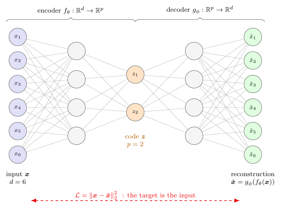
Figure 12.1: An undercomplete autoencoder in the layer notation of Section Notation and the feed-forward pass, with \(d=6\) and \(p=2\). Read left to right it is an ordinary feed-forward network of Figure 8.5; what makes it an autoencoder is the dashed arrow at the bottom, which says that the target of example \(n\) is example \(n\) itself. No labels enter anywhere, which is the content of the word self-supervised. Everything the network knows about \(\bm{x}\) after the encoder must pass through the two orange units, and the reconstruction is built from those two numbers alone.
The layer that produces \(\bm{z}\) is the bottleneck, and its width \(p\) is the single most important architectural choice. Three regimes are worth naming.
Undercomplete, \(p<d\). The code cannot hold the input, so the network must decide what to discard. This is the case in which reconstruction forces compression, and it is the case the first half of this chapter analyses exactly.
Complete, \(p=d\). Nothing is forced.
Overcomplete, \(p\ge d\). The identity is available: \(f=g=\mathrm{id}\) gives zero error and learns nothing. Something other than the bottleneck must supply the constraint, and Section Regularised autoencoders is about what.
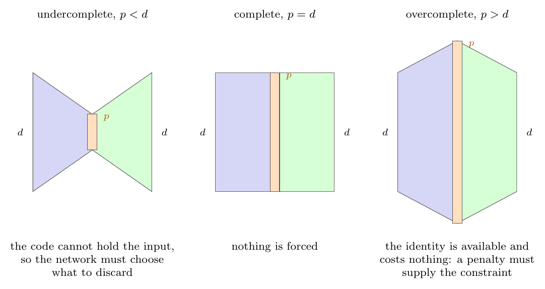
Figure 12.2: The three regimes of the bottleneck width, drawn as the width of the representation against depth. Only the first compresses. In the second and third the map \(g\circ f=\mathrm{id}\) is available and achieves zero reconstruction error while learning nothing whatever about the data, so the constraint that makes the network useful has to come from somewhere other than the architecture – which is what Section Regularised autoencoders supplies. The orange bar is the code layer in each case.
Figure 12.2 contrasts the three. In practice the two halves are usually mirrored: a decoder whose layer widths are those of the encoder in reverse. This is a convention rather than a requirement, but it is a sensible one, and it makes the parameter counts of the two halves match.
Activations and the cost. The hidden layers use whatever Chapter 8 recommends. The output layer is the one that needs thought, and it should be chosen to match the range of the data.
If the inputs are unbounded real numbers, the output activation is the identity and the cost is Eq. (12.2). If they have been scaled to \([0,1]\) – pixel intensities, most commonly – a logistic output is natural, and the binary cross-entropy
is then often preferred to the squared error, because it is the negative log-likelihood of a Bernoulli model and it penalises confident mistakes near the ends of the range much more heavily. A ReLU output is appropriate when the data are non-negative and unbounded, and a linear output is wrong for bounded data because it can predict outside the range.
12.2. Reconstruction, projection and representation#
Before the analysis it is worth being precise about what is being asked. The optimisation is over function classes: let \(\mathcal{F}\) be a class of encoders and \(\mathcal{G}\) a class of decoders, and solve
If \(\mathcal{F}\) and \(\mathcal{G}\) are linear this is a constrained quadratic problem with a closed-form solution. If they are neural networks it is non-convex and highly expressive, and we are back in the territory of Chapter 4.
A theme that will recur is the decomposition
which says that minimising reconstruction error and maximising captured variance are the same problem seen from two sides. For linear autoencoders this is exact and we prove it below; Figure 12.3 is the proof in one picture, since the decomposition is Pythagoras’ theorem applied at each data point and summed.
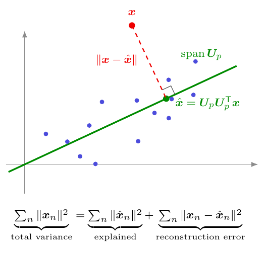
Figure 12.3: What a linear autoencoder does, in \(d=2\) with \(p=1\), on centred data – which is why the subspace passes through the origin. Lemma 12.1 says that the best reconstruction of a given rank can always be taken to be an orthogonal projection, so \(\hat{\bm{x}}\) is the foot of the perpendicular from \(\bm{x}\) to the subspace, and Theorem 12.5 identifies the subspace that minimises the total squared residual as the principal one. The right angle is the whole of Eq. (12.5): Pythagoras at every data point, summed, splits the total variance into an explained part and a reconstruction error, so making one small is exactly making the other large. A nonlinear autoencoder replaces the straight line by a curve and changes nothing else in the picture.
Reconstruction is not representation
Equation (12.2) scores the network on \(\hat{\bm{x}}\), not on \(\bm{z}\). Nothing in it asks the code to be interpretable, smooth, disentangled or ordered, and Section Beyond PCA shows an example in which the reconstruction is excellent and the code is nevertheless a poor coordinate for the data. A low reconstruction error is evidence that the information survived the bottleneck. It is not evidence that it survived in a useful form.
12.3. The linear autoencoder#
Take the encoder and decoder to be linear and without biases,
so that the reconstruction map is \(\hat{\bm{x}}=\bm{A}\bm{x}\) with \(\bm{A}=\bm{W}_d^{\mathsf{T}}\bm{W}_e^{\mathsf{T}}\). Since \(\bm{A}\) factors through \(\mathbb{R}^{p}\),
Dropping the biases costs nothing provided the data are centred, which we assume throughout: replace \(\bm{x}_n\) by \(\bm{x}_n-\bar{\bm{x}}\). With the data arranged as the rows of \(\bm{X}\in\mathbb{R}^{N\times d}\), the training problem is
The equality is the first substantive step: any matrix of rank at most \(p\) can be written as \(\bm{W}_d^{\mathsf{T}}\bm{W}_e^{\mathsf{T}}\) by taking a rank factorisation, so optimising over the two factors is the same as optimising over their product subject to the rank bound. Linear autoencoder training is a rank-constrained approximation problem.
Write \(\bm{S}=\bm{X}^{\mathsf{T}}\bm{X}/N\) for the empirical covariance, and let its eigendecomposition be
with \(\bm{U}\) orthogonal and \(\bm{U}_p=[\bm{u}_1,\dots,\bm{u}_p]\) its first \(p\) columns. Recall from Chapter 1 that \(\bm{S}\) is symmetric positive semi-definite, so such a decomposition exists with real non-negative eigenvalues.
12.3.1. Reduction to an orthogonal projector#
Lemma 12.1 (The optimum may be taken to be an orthogonal projector)
Let \(\bm{A}\) have rank at most \(p\) and let \(\bm{P}\) be the orthogonal projector onto the row space of \(\bm{A}\) (equivalently, onto the image of \(\bm{A}^{\mathsf{T}}\)). Then \(\operatorname{rank}(\bm{P})\le p\) and
Proof
Let \(\mathcal{M}\) be the row space of \(\bm{A}\), of dimension at most \(p\). For each \(n\), the row \(\bm{x}_n^{\mathsf{T}}\bm{A}\) lies in \(\mathcal{M}\), and \(\bm{x}_n^{\mathsf{T}}\bm{P}\) is by definition the point of \(\mathcal{M}\) closest to \(\bm{x}_n\) in the Euclidean norm. Hence
and summing over \(n\) gives Eq. (12.10), the Frobenius norm being the sum over rows of the squared Euclidean norms.
Lemma 12.1 is what makes the whole analysis possible. It replaces an optimisation over all rank-\(p\) matrices, a set with \(p(2d-p)\) parameters and no useful structure, by an optimisation over rank-\(p\) orthogonal projectors, which are parameterised by a Grassmannian – that is, by a choice of subspace and nothing else. Every orthogonal projector of rank \(p\) has the form
with \(\bm{B}\) an orthonormal basis of the subspace.
12.3.2. Reduction to a trace maximisation#
Lemma 12.2 (Error equals variance not captured)
With \(\bm{P}=\bm{B}\bm{B}^{\mathsf{T}}\) as in Eq. (12.11),
Minimising the reconstruction error is therefore equivalent to maximising \(\operatorname{Tr}(\bm{B}^{\mathsf{T}}\bm{S}\bm{B})\) subject to \(\bm{B}^{\mathsf{T}}\bm{B}=\bm{I}_p\).
Proof
Expand the norm as a trace and use \(\bm{P}^{\mathsf{T}}=\bm{P}\) and \(\bm{P}^{2}=\bm{P}\):
using \(\bm{X}^{\mathsf{T}}\bm{X}=N\bm{S}\). Idempotence and cyclicity of the trace give \(\operatorname{Tr}[(\bm{I}-\bm{P})\bm{S}(\bm{I}-\bm{P})] =\operatorname{Tr}[\bm{S}(\bm{I}-\bm{P})] =\operatorname{Tr}(\bm{S})-\operatorname{Tr}(\bm{S}\bm{P})\), and finally \(\operatorname{Tr}(\bm{S}\bm{B}\bm{B}^{\mathsf{T}}) =\operatorname{Tr}(\bm{B}^{\mathsf{T}}\bm{S}\bm{B})\).
Equation (12.12) is Eq. (12.5) made precise: \(\operatorname{Tr}(\bm{S})\) is the total variance, fixed by the data, and \(\operatorname{Tr}(\bm{B}^{\mathsf{T}}\bm{S}\bm{B})\) is the variance captured by the subspace.
12.3.3. The variational characterisation#
It remains to maximise \(\operatorname{Tr}(\bm{B}^{\mathsf{T}}\bm{S}\bm{B})\). We do the case \(p=1\) by a Lagrange multiplier, which is where the eigenvalue problem appears, and then state the general case.
Proposition 12.3 (The first direction)
The maximiser of \(\bm{w}^{\mathsf{T}}\bm{S}\bm{w}\) subject to \(\|\bm{w}\|_2=1\) is the eigenvector \(\bm{u}_1\) of \(\bm{S}\) belonging to the largest eigenvalue \(\lambda_1\), and the maximum equals \(\lambda_1\).
Proof
Without the constraint the objective is unbounded, since scaling \(\bm{w}\) scales it quadratically; the constraint is therefore essential. Impose it with a multiplier and maximise
By the matrix-calculus identities of Section Derivatives with respect to vectors and matrices,
so every stationary point is an eigenvector of \(\bm{S}\). Left-multiplying by \(\bm{w}^{\mathsf{T}}\) and using \(\|\bm{w}\|=1\) gives \(\bm{w}^{\mathsf{T}}\bm{S}\bm{w}=\lambda\): the value of the objective at a stationary point is the corresponding eigenvalue. The maximum is therefore attained at the largest one.
The direction that maximises the variance of the projected data is an eigenvector of the covariance matrix, and the variance it captures is the eigenvalue. That single sentence is the content of principal component analysis.
Theorem 12.4 (Ky Fan)
Let \(\bm{S}\) be symmetric with eigenvalues \(\lambda_1\ge\dots\ge\lambda_d\) and eigenvectors \(\bm{u}_1,\dots,\bm{u}_d\). Then
attained at \(\bm{B}=\bm{U}_p\), and at \(\bm{B}=\bm{U}_p\bm{Q}\) for any orthogonal \(\bm{Q}\in\mathbb{R}^{p\times p}\).
Proof
Write \(\bm{C}=\bm{U}^{\mathsf{T}}\bm{B}\), which also satisfies \(\bm{C}^{\mathsf{T}}\bm{C}=\bm{I}_p\) since \(\bm{U}\) is orthogonal. Then
The coefficients \(m_i\) satisfy two constraints. Each row of \(\bm{C}\) has norm at most one, because \(\bm{C}\) has orthonormal columns and may be completed to an orthogonal matrix, so \(0\le m_i\le1\); and \(\sum_i m_i=\|\bm{C}\|_F^{2}=\operatorname{Tr}(\bm{C}^{\mathsf{T}}\bm{C})=p\). Maximising the linear functional \(\sum_i\lambda_i m_i\) over the polytope \(\{0\le m_i\le1,\ \sum_i m_i=p\}\) puts all the available mass on the largest \(\lambda_i\), giving \(m_1=\dots=m_p=1\) and the rest zero, hence the value \(\sum_{i\le p}\lambda_i\). This is attained by \(\bm{C}=[\bm{I}_p;\bm{0}]\), that is \(\bm{B}=\bm{U}_p\), and the value is unchanged by \(\bm{B}\to\bm{B}\bm{Q}\) with \(\bm{Q}\) orthogonal since \(\operatorname{Tr}(\bm{Q}^{\mathsf{T}} \bm{B}^{\mathsf{T}}\bm{S}\bm{B}\bm{Q}) =\operatorname{Tr}(\bm{B}^{\mathsf{T}}\bm{S}\bm{B})\).
12.3.4. The theorem#
Assembling Lemmas 12.1 and 12.2 with Theorem 12.4 gives the result.
Theorem 12.5 (Linear autoencoders perform PCA)
Let \(\bm{X}\in\mathbb{R}^{N\times d}\) be centred with empirical covariance \(\bm{S}=\bm{X}^{\mathsf{T}}\bm{X}/N\), eigenvalues \(\lambda_1\ge\dots\ge\lambda_d\ge0\) and eigenvectors \(\bm{U}\). Consider the linear autoencoder (12.6) with bottleneck width \(p\le d\) trained on the reconstruction error (12.2). Then:
the minimum of the reconstruction error is
\[ \min_{\bm{W}_e,\bm{W}_d}\frac{1}{N} \left\|\bm{X}-\bm{X}\bm{W}_e\bm{W}_d\right\|_F^{2} = \sum_{i=p+1}^{d}\lambda_i,\tag{12.14} \]the sum of the discarded eigenvalues;
at any global minimiser the product satisfies \(\bm{W}_e\bm{W}_d=\bm{U}_p\bm{U}_p^{\mathsf{T}}\), the orthogonal projector onto the leading eigenspace, and the reconstruction is therefore identical to the rank-\(p\) PCA reconstruction \(\hat{\bm{x}} =\bm{U}_p\bm{U}_p^{\mathsf{T}}\bm{x}\);
the column space of \(\bm{W}_e\) equals \(\operatorname{span}\{\bm{u}_1,\dots,\bm{u}_p\}\), assuming \(\lambda_p>\lambda_{p+1}\).
Proof
By Eq. (12.8) the problem is over matrices of rank at most \(p\); by Lemma 12.1 the infimum is attained on orthogonal projectors, which by Eq. (12.11) are parameterised by \(\bm{B}\) with orthonormal columns; by Lemma 12.2 the objective becomes \(N[\operatorname{Tr}(\bm{S}) -\operatorname{Tr}(\bm{B}^{\mathsf{T}}\bm{S}\bm{B})]\); and by Theorem 12.4 the second trace is maximised at \(\sum_{i\le p}\lambda_i\) with \(\bm{B}=\bm{U}_p\bm{Q}\). Since \(\operatorname{Tr}(\bm{S})=\sum_i\lambda_i\), the minimum value is \(N\sum_{i>p}\lambda_i\), which after division by \(N\) is Eq. (12.14). The optimal projector is \(\bm{B}\bm{B}^{\mathsf{T}}=\bm{U}_p\bm{Q}\bm{Q}^{\mathsf{T}}\bm{U}_p^{\mathsf{T}} =\bm{U}_p\bm{U}_p^{\mathsf{T}}\), independent of \(\bm{Q}\), which gives (ii); the gap condition \(\lambda_p>\lambda_{p+1}\) makes the maximising subspace unique and gives (iii).
The result deserves a moment’s reflection, and one qualification. Theorem 12.5 characterises the global minimum; it says nothing about what gradient descent finds, and for a non-convex objective those are different questions. What closes the gap is that this particular objective has no bad places to get stuck.
Proposition 12.6 (The landscape has no spurious minima)
Assume \(\lambda_1>\dots>\lambda_d>0\). Every critical point of the linear autoencoder objective (12.2) with \(\bm{W}_e\bm{W}_d\) of rank exactly \(p\) has \(\bm{W}_e\bm{W}_d=\bm{U}_{\mathcal{I}}\bm{U}_{\mathcal{I}}^{\mathsf{T}}\) for some index set \(\mathcal{I}\subset\{1,\dots,d\}\) with \(|\mathcal{I}|=p\). Such a point is a global minimum if and only if \(\mathcal{I}=\{1,\dots,p\}\); every other choice is a saddle. There are no local minima that are not global.
Proof
Stationarity of Eq. (12.2) in \(\bm{W}_d\) gives \(\bm{W}_e^{\mathsf{T}}\bm{S}(\bm{I}-\bm{W}_e\bm{W}_d)=\bm{0}\) and in \(\bm{W}_e\) gives \(\bm{S}(\bm{I}-\bm{W}_e\bm{W}_d)\bm{W}_d^{\mathsf{T}}=\bm{0}\); together these force \(\bm{\Pi}=\bm{W}_e\bm{W}_d\) to satisfy \(\bm{\Pi}\bm{S}=\bm{S}\bm{\Pi}=\bm{\Pi}\bm{S}\bm{\Pi}\), so \(\bm{\Pi}\) is a projector commuting with \(\bm{S}\) and therefore projects onto a span of eigenvectors, indexed by some \(\mathcal{I}\). The objective value there is \(\sum_{i\notin\mathcal{I}}\lambda_i\) by the argument of Theorem 12.5.
Now suppose \(\mathcal{I}\neq\{1,\dots,p\}\), so there are indices \(j\notin\mathcal{I}\) and \(k\in\mathcal{I}\) with \(\lambda_j>\lambda_k\). Consider the curve of projectors obtained by rotating \(\bm{u}_k\) towards \(\bm{u}_j\) by an angle \(\vartheta\) inside their two-dimensional span; the objective along it is
since the rotation exchanges a fraction \(\sin^{2}\vartheta\) of the weight on \(\lambda_k\) for the same fraction on \(\lambda_j\). Thus \(E'(0)=0\) – confirming criticality – and \(E''(0)=-2(\lambda_j-\lambda_k)<0\): the point is a strict maximum along this direction while being a minimum along the \(GL(p)\) orbit of Proposition 12.7, hence a saddle. Only \(\mathcal{I}=\{1,\dots,p\}\) admits no such pair, and by Theorem 12.5 it is the global minimum.
This is what licenses the informal statement that a linear autoencoder “does PCA”. A neural network trained by gradient descent on a non-convex objective is guaranteed to land on a classical, spectrally characterised answer – not because the objective is convex, which it is not, but because its only non-global critical points are saddles, which first-order methods with noise leave. It is essentially the only architecture in this book for which we can say that, and Section PyTorch and TensorFlow measures how well the promise is kept in practice.
Proposition 12.7 (What the autoencoder does not recover)
If \((\bm{W}_e,\bm{W}_d)\) is a global minimiser then so is \((\bm{W}_e\bm{M},\bm{M}^{-1}\bm{W}_d)\) for every invertible \(\bm{M}\in\mathbb{R}^{p\times p}\). Consequently the individual weights are determined only up to \(GL(p)\): the autoencoder recovers the principal subspace, not the principal directions, and its codes are not in general uncorrelated, ordered by variance, or of unit norm.
Proof
\((\bm{W}_e\bm{M})(\bm{M}^{-1}\bm{W}_d)=\bm{W}_e\bm{W}_d\), so the reconstruction and hence the cost are unchanged.
This is the practical difference between running PCA and training a linear autoencoder, and it is easy to overlook. PCA delivers an orthonormal basis ordered by variance, so that truncating to \(q<p\) components is meaningful and the components are uncorrelated by construction. A linear autoencoder delivers some basis of the same subspace, in no particular order, generally not orthogonal. If the directions matter, use PCA; if only the subspace matters, either will do, and PCA is faster.
Relation to Eckart-Young and the SVD
Theorem 12.5 is a close relative of the Eckart-Young theorem of Section The singular value decomposition, which states that the best rank-\(p\) approximation to \(\bm{X}\) in the Frobenius norm is obtained by truncating its singular value decomposition, with error \(\sum_{i>p}\sigma_i^{2}\). The two are connected by \(\sigma_i^{2}=N\lambda_i\): the singular values of the centred data matrix are the square roots of \(N\) times the eigenvalues of the covariance. The difference is that Eckart-Young approximates \(\bm{X}\) by any low-rank matrix, while the autoencoder is constrained to approximate each \(\bm{x}_n\) by a fixed linear map applied to \(\bm{x}_n\) itself. That the two give the same answer is a consequence of Lemma 12.1. In practice one computes PCA by the SVD of \(\bm{X}\) rather than by eigendecomposing \(\bm{S}\), for the conditioning reason given in Section The singular value decomposition: forming \(\bm{X}^{\mathsf{T}}\bm{X}\) squares the condition number.
12.4. Verifying the theorem#
The chapter’s code is the network of Chapter 8 with the target set equal to the input. Nothing else changes, which is the point.
def ae_forward(P, X, acts):
    """Returns the reconstruction and the cache; X has shape (N, d)."""
    A = [X]; Z = []
    a = X
    for l, (W, b) in enumerate(P):
        z = a @ W + b
        Z.append(z)
        a = ACT[acts[l]][0](z)
        A.append(a)
    return a, (A, Z)


def ae_backward(P, cache, Xhat, X, acts):
    """Backpropagation with the target equal to the input, Eq. (12.cost)."""
    A, Z = cache
    n = X.shape[0]
    g = [[np.zeros_like(W), np.zeros_like(b)] for W, b in P]
    delta = (Xhat - X) / n * ACT[acts[-1]][1](Z[-1])
    for l in reversed(range(len(P))):
        g[l][0] = A[l].T @ delta
        g[l][1] = delta.sum(axis=0)
        if l > 0:
            delta = (delta @ P[l][0].T) * ACT[acts[l - 1]][1](Z[l - 1])
    return g
Checking every parameter against central differences, for three architectures:
  [6, 3, 6]          ['identity', 'identity']
      max relative error 8.71e-09   max absolute error 6.93e-10
      (9 entries had gradient 0 and were checked absolutely)
  [6, 4, 2, 4, 6]    ['tanh', 'tanh', 'tanh', 'sigmoid']
      max relative error 1.91e-06   max absolute error 6.19e-10
  [6, 3, 6]          ['relu', 'identity']
      max relative error 2.12e-08   max absolute error 7.35e-10
A relative check is meaningless on a gradient that is zero
The first line above reports nine parameters excluded from the relative comparison. They are the biases of a linear autoencoder on centred data, whose gradients are exactly zero – the analytic value came out as \(4.9\times10^{-17}\) and the central difference as \(-4.4\times10^{-10}\), pure subtraction noise. Their ratio is \(\bigO(1)\) and means nothing. This is the same lesson as the ReLU kink of Section Verifying the implementation, in a different disguise: a gradient checker needs an absolute test as well as a relative one, and needs to know which to apply where.
Now the theorem. We generate \(600\) points in \(\mathbb{R}^{8}\) lying near a three-dimensional subspace, plus isotropic noise, and train a \([8,3,8]\) linear autoencoder by Adam. Against the predictions of Theorem 12.5 and Proposition 12.7:
AE  reconstruction error : 0.308313
PCA reconstruction error : 0.306324
eigenvalue tail          : 0.306324
AE/PCA error ratio       : 1.006493
principal angles (deg)   : [0.0684 0.1851 0.318 ]
||W_e W_d - Pi||_F       : 9.895e-03
singular values of W_e W_d: [1.0033 1.0007 0.9989 1.166e-16 6.462e-17
                             5.420e-17 3.645e-17 1.840e-18]
||W_e - U_p||_F          : 1.8737  (NOT small)
dist(W_e, span U_p)      : 2.466e-03  (small: same subspace)
Every line is a prediction confirmed. The PCA reconstruction error and the eigenvalue tail agree to all six digits printed, which is Eq. (12.14). The autoencoder gets to within \(0.65\%\) of that floor and does not cross it. The singular values of \(\bm{W}_e\bm{W}_d\) are three ones and five zeros to machine precision, so the trained product really is an orthogonal projector of rank three, as Lemma 12.1 said it would be. The principal angles between the learned subspace and the leading eigenspace are a fifth of a degree.
And the last two lines are Proposition 12.7 in numbers. The distance from \(\bm{W}_e\) to \(\bm{U}_p\) is \(1.87\), which is not small – the weights are nowhere near the eigenvectors – while the distance from \(\bm{W}_e\) to the span of \(\bm{U}_p\) is \(2.5\times10^{-3}\). Same subspace, different basis. A reader who trained a linear autoencoder expecting to read principal directions off the encoder weights would get nonsense, and the reconstruction error would give no hint of it.
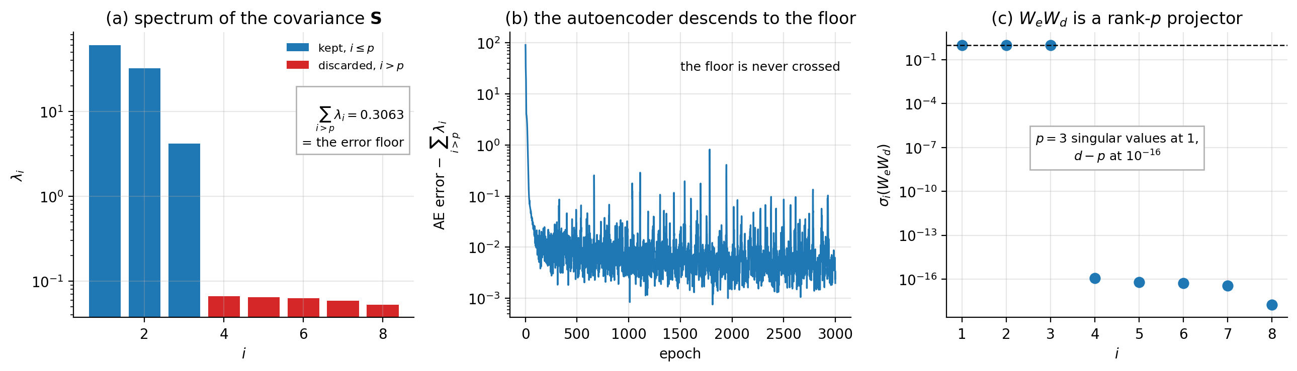
Figure 12.4: (a) The eigenvalue spectrum of \(\bm{S}\) on a logarithmic scale; the red bars are the discarded eigenvalues whose sum is the error floor of Eq. (12.14). (b) The autoencoder’s reconstruction error minus that floor during training: it approaches zero from above and never crosses, as Theorem 12.5 guarantees. (c) Singular values of the trained product \(\bm{W}_e\bm{W}_d\): exactly \(p=3\) of them equal one and the remaining \(d-p=5\) are at the level of rounding, confirming that the learned map is an orthogonal projector of rank \(p\).
12.5. Beyond PCA#
PCA finds the best linear subspace. Many data sets do not lie near one: images of a rotating object, molecular conformations, solutions of a nonlinear partial differential equation parameterised by a boundary condition, speech. These lie near a curved manifold, and no linear subspace of the manifold’s dimension will follow it.
Replacing the linear maps of Eq. (12.6) by the deep networks of Chapter 8,
buys the ability to bend. It also costs the entire analysis of Section The linear autoencoder: the problem becomes non-convex, no closed form is available, and we are back to gradient descent with no guarantee of a global optimum.
What replaces the projector. If \(f\) and \(g\) are differentiable then near a point \(\bm{x}_0\), with \(\bm{z}_0=f(\bm{x}_0)\),
so the product of Jacobians \(\bm{J}_g\bm{J}_f\) is the local reconstruction operator. It plays the role that \(\bm{W}_e\bm{W}_d\) played in the linear case, with the crucial difference that it now varies from point to point. A nonlinear autoencoder is, to first order, a projector onto the tangent space of the data manifold, chosen afresh at every location.
Measuring the difference. We put \(800\) training and \(400\) test points on a one-dimensional curve — a helix — embedded in \(\mathbb{R}^{3}\) with small isotropic noise, and compare PCA against a \([3,16,p,16,3]\) autoencoder with \(\tanh\) hidden layers.
\noalign{} \(p\) |
Method |
train error |
test error |
|---|---|---|---|
\noalign{}\noalign{} \(1\) |
PCA |
\(0.7855\) |
\(0.7914\) |
\(1\) |
nonlinear autoencoder |
\(0.1511\) |
\(\mathbf{0.2012}\) |
\noalign{}\noalign{} \(2\) |
PCA |
\(0.3208\) |
\(0.3316\) |
\(2\) |
nonlinear autoencoder |
\(0.0020\) |
\(\mathbf{0.0062}\) |
\noalign{} |
Table 12.1: A one-dimensional curved manifold in \(\mathbb{R}^{3}\). Errors are \(\|\bm{x}-\hat{\bm{x}}\|^{2}\) averaged over points, and the autoencoder figures are means over three seeds. The total variance per point is \(1.287\).
At \(p=1\) the autoencoder is four times more accurate than PCA; at \(p=2\) it is fifty times more accurate. The sharpest way to put it is to compare across rows: the one-dimensional nonlinear code, at \(0.2012\), beats the two-dimensional linear one, at \(0.3316\). Curvature is worth more than a dimension here, and Theorem 12.5 tells us exactly why PCA cannot do better – its error is fixed by the eigenvalue tail, and no amount of training changes it.
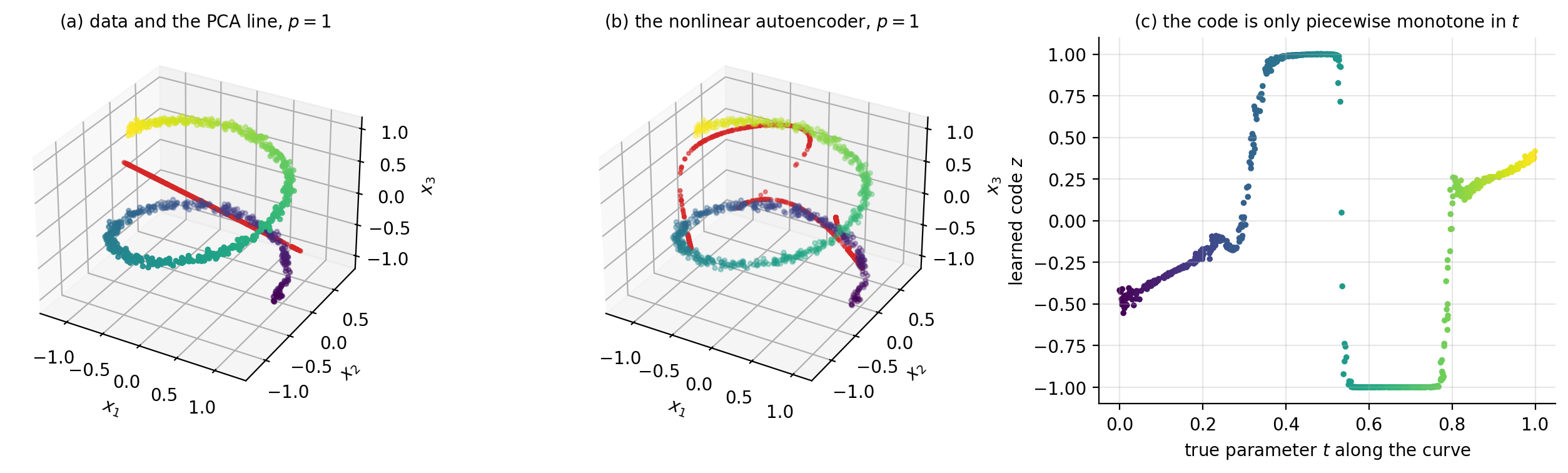
Figure 12.5: (a) The data, coloured by position along the curve, with the one-dimensional PCA reconstruction in red: a straight line through a helix. (b) The same data with the one-dimensional nonlinear autoencoder reconstruction, which follows the curve. (c) The learned code \(z\) against the true parameter \(t\). The relation is monotone in stretches but saturates at \(\pm1\) and jumps: the reconstruction is good and the coordinate is not.
Panel (c) of Figure 12.5 is the honest part, and it is the notebox of Section Reconstruction, projection and representation made visible. The autoencoder reconstructs the helix well, but the code it uses to do so is not a faithful coordinate along the curve: it saturates against the limits of the \(\tanh\) and jumps between branches. Nothing in Eq. (12.2) asked for a good coordinate, so nothing delivered one. If the latent variable is to be interpreted – as a reaction coordinate, an order parameter, a physical parameter of the system – then reconstruction error alone is the wrong objective, and one of the regularisers of the next section, or the probabilistic treatment of Section The probabilistic view: PPCA, must be brought in.
12.6. Regularised autoencoders#
The bottleneck is one way to prevent an autoencoder from learning the identity. It is not the only way, and an overcomplete autoencoder with \(p\ge d\) needs another, since \(g\circ f=\mathrm{id}\) is available and costs nothing. All three constructions below add a penalty to Eq. (12.2) and can replace the bottleneck entirely.
Denoising autoencoders.
Corrupt the input and ask for the clean version back. With \(\tilde{\bm{x}}=\bm{x}+\bm{\varepsilon}\),
Copying the input is now actively harmful, because the input is wrong. The network must instead learn where the data are, so as to move a corrupted point back onto them. There is a striking statistical reading of this: for small Gaussian corruption the optimal reconstruction satisfies
so the displacement the network applies is proportional to the score of the data density. A denoising autoencoder is, without being told so, an estimator of \(\nabla\log p\) – which is exactly the object that score-based and diffusion generative models are built on.
Sparse autoencoders.
Penalise the code rather than the reconstruction:
The \(\ell_1\) penalty is the one that produced exact zeros in Section The Lasso, and it does the same here: each input activates only a few latent units, and those units tend to become recognisable feature detectors. The construction is close kin to dictionary learning and sparse coding.
Contractive autoencoders.
Penalise the sensitivity of the encoder:
The two terms pull in opposite directions and the geometry of the compromise is the point. Reconstruction requires the encoder to be sensitive to displacements along the data manifold, since those change which point is being encoded. The penalty asks it to be insensitive in all directions. The optimum keeps sensitivity where it is needed and suppresses it elsewhere, so that \(\bm{J}_f\) ends up large on the tangent space of the manifold and small on the normal directions. The encoder learns the manifold’s tangent structure. Figure 12.6 draws the denoising and the contractive geometry next to one another, which is the quickest way to see why the two are so nearly the same construction.
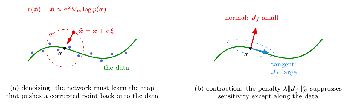
Figure 12.6: The geometry behind the two regularisers of Section Regularised autoencoders, drawn for data concentrated near a curve in the plane. (a) Denoising, Eq. (12.17): the corrupted input \(\tilde{\bm{x}}\) is displaced off the data by an amount of order \(\sigma\), and the network is scored on how well it recovers the clean \(\bm{x}\), so it must learn the map that points back towards where the data are. Equation (12.18) identifies that map, to leading order, with the score \(\nabla_{\bm{x}}\log p\). (b) Contraction, Eq. (12.20): reconstruction needs the encoder to respond to displacements along the data, while the penalty asks it to respond to nothing at all; the compromise keeps \(\bm{J}_f\) large on the tangent and small on the normal, so the ellipse of responses is flattened onto the manifold. Proposition 12.8 makes the resemblance precise to order \(\sigma^{2}\), with the one caveat recorded there: the denoising penalty falls on \(\bm{J}_r\), the sensitivity of the round trip, and not on \(\bm{J}_f\).
The last sentence of the notebox below says these regularisers are “the same idea”. For two of them that is a theorem rather than an impression.
Proposition 12.8 (Denoising is contraction, to second order)
Let \(r=g\circ f\) be the reconstruction map and let the denoising objective (12.17) use additive noise \(\tilde{\bm{x}}=\bm{x}+\sigma\bm{\xi}\) with \(\mathbb{E}[\bm{\xi}]=\bm{0}\) and \(\mathbb{E}[\bm{\xi}\bm{\xi}^{\mathsf{T}}]=\bm{I}\). If \(r\) is twice continuously differentiable then
where \(\bm{J}_r=\partial r/\partial\bm{x}\). Training a denoising autoencoder at noise level \(\sigma\) is therefore, to leading order, training a plain autoencoder with the contractive penalty (12.20) at \(\lambda=\sigma^{2}\) – applied to the whole reconstruction rather than to the encoder alone.
Proof
Taylor-expand \(r(\bm{x}+\sigma\bm{\xi}) =r(\bm{x})+\sigma\bm{J}_r\bm{\xi}+\bigO(\sigma^{2})\) and substitute:
Taking the expectation, the middle term vanishes because \(\mathbb{E}[\bm{\xi}]=\bm{0}\), and the last one is \(\sigma^{2}\operatorname{Tr}(\bm{J}_r^{\mathsf{T}}\bm{J}_r) =\sigma^{2}\|\bm{J}_r\|_F^{2}\), because \(\mathbb{E}[\bm{\xi}\bm{\xi}^{\mathsf{T}}]=\bm{I}\). The neglected terms are \(\bigO(\sigma^{3})\) since the \(\bigO(\sigma^{2})\) term of the expansion enters the square multiplied by the first-order one.
Equation (12.21) explains why the two constructions behave so similarly in practice, and it also explains why they are not identical: the denoising penalty falls on \(\bm{J}_r\), the sensitivity of the round trip, while Eq. (12.20) penalises \(\bm{J}_f\), the sensitivity of the encoder alone. A decoder that amplifies can hide from the second and not from the first. It also predicts what the noise level buys: doubling \(\sigma\) quadruples the effective \(\lambda\), so the reconstruction error should degrade smoothly rather than sharply, which is what Section The regularised variants, measured finds.
These are all the same idea
A bottleneck restricts the code by dimension; sparsity restricts it by how many coordinates may be non-zero; contraction restricts it by how fast it may vary; denoising restricts it by requiring robustness. In each case the network is prevented from being the identity and must spend its capacity on structure instead. This is the bias-variance trade-off of Section The bias-variance tradeoff appearing once more, with the regulariser choosing which functions are cheap.
12.7. The probabilistic view: PPCA#
Everything so far has been deterministic: a code \(\bm{z}=f(\bm{x})\) and a reconstruction \(\hat{\bm{x}}=g(\bm{z})\). A probabilistic autoencoder replaces these by a latent-variable model \(p_\theta(\bm{x},\bm{z})=p_\theta(\bm{x}\mid\bm{z})p(\bm{z})\), turning representation learning into statistical inference of the kind Chapter 2 set up.
The linear case again has a complete answer. Probabilistic PCA assumes
so that \(p(\bm{x}\mid\bm{z})=\mathcal{N}(\bm{W}\bm{z}+\bm{\mu}, \sigma^{2}\bm{I}_d)\). Integrating out the latent variable, which is a Gaussian marginalisation and therefore exact,
The model therefore describes the covariance as a low-rank term plus isotropic noise, \(\bm{\Sigma}=\bm{W}\bm{W}^{\mathsf{T}}+\sigma^{2}\bm{I}\), which is the probabilistic statement of “low-dimensional structure plus measurement error”.
Maximum-likelihood estimation in this model, worked out by Tipping and Bishop [tipping1999], gives a loading matrix whose column space is exactly the principal subspace, and \(\hat{\sigma}^{2}\) equal to the average of the discarded eigenvalues,
Compare Eq. (12.14): the same eigenvalue tail that bounded the autoencoder’s reconstruction error reappears as the estimated noise variance. As \(\sigma^{2}\to0\) the model degenerates to the deterministic projection, and PPCA becomes ordinary PCA. Once again \(\bm{W}\) is determined only up to an orthogonal factor, for the reason given in Proposition 12.7.
The gain is what a probabilistic model always gives: a likelihood, hence a principled way to choose \(p\); a generative model one can sample from; and a proper treatment of missing data. Replacing the linear map in Eq. (12.22) by a neural network, and the exact marginalisation by a variational bound, gives the variational autoencoder, which belongs to a later discussion of generative models.
12.8. Implementations#
12.8.1. Our own#
The complete autoencoder is the code of Section Verifying the theorem with a list of layer widths and activations. A deep autoencoder on the helix of Table 12.1 is four lines:
acts = ["tanh", "tanh", "tanh", "identity"]
P = init_ae([3, 16, 1, 16, 3], acts, np.random.default_rng(0))
P, hist = train_ae(P, X, acts, n_epoch=600, batch=32, gamma=5e-3, Xval=Xte)
Z = encode(P, X, acts, layer=2)          # the code: run the first two layers
Setting \verb!acts = [“identity”, “identity”]! and \verb!sizes = [d, p, d]! recovers the linear autoencoder of Theorem 12.5, and \verb!pca(X, p)! in the same module returns the projector, the loadings and the eigenvalues for comparison. The two are worth running side by side once.
Centre the data
Theorem 12.5 assumes it, and PCA without it finds the direction of the mean rather than the direction of greatest variance. Scikit-learn’s \verb!PCA! centres internally; our \verb!pca! does so too; a hand-written implementation or a neural network without biases does not. If the features have incomparable units, standardise as well as centre, or the covariance will be dominated by whichever feature happens to be measured in small units.
12.8.2. PyTorch and TensorFlow#
Two things are worth doing in a library. The first is to check that it computes what we derived: one set of weights pushed into our code, into PyTorch and into Keras should give the same reconstruction and the same gradients. The second, and the more interesting, is to put Theorem 12.5 and Proposition 12.6 to the test – to train a linear autoencoder by Adam and ask whether it really lands on the principal subspace, and whether it really fails to land on the principal basis.
The conversion is trivial here, which is worth saying because it was not in Chapters 10 and 11: Keras stores a dense weight as \((n_{\mathrm{in}},n_{\mathrm{out}})\), exactly as our code does, and only PyTorch transposes. With that one transposition:
=== 1. one autoencoder, identical weights ===
  reconstruction max |ours - torch| : 3.886e-16
  reconstruction max |ours - keras| : 3.608e-16
  our cost, Eq. (12.cost)           : 5.781582466015
  torch cost                        : 5.781582466015
   layer      shape          |ours - torch| W    |ours - torch| b
   0   (12, 8)                  2.220e-16           6.765e-17
   1   (8, 3)                   2.220e-16           5.551e-17
   2   (3, 8)                   1.110e-16           1.388e-16
   3   (8, 12)                  8.327e-17           5.898e-17
  worst disagreement: 2.220e-16
so the network of Section Our own and the two libraries are the same function, and its gradients are the same gradients.
The listings below are the standard constructions. The first is a linear autoencoder, which should reproduce PCA.
import numpy as np
import tensorflow as tf
from tensorflow import keras

# three-dimensional data lying near a plane
np.random.seed(4)
def generate_3d_data(m, w1=0.1, w2=0.3, noise=0.1):
    angles = np.random.rand(m) * 3 * np.pi / 2 - 0.5
    data = np.empty((m, 3))
    data[:, 0] = np.cos(angles) + np.sin(angles)/2 + noise*np.random.randn(m)/2
    data[:, 1] = np.sin(angles) * 0.7 + noise * np.random.randn(m) / 2
    data[:, 2] = data[:, 0]*w1 + data[:, 1]*w2 + noise*np.random.randn(m)
    return data

X_train = generate_3d_data(60)
X_train = X_train - X_train.mean(axis=0, keepdims=True)   # centre: see the notebox

# no activations anywhere: this is Eq. (12.linae)
encoder = keras.models.Sequential([keras.layers.Dense(2, input_shape=[3])])
decoder = keras.models.Sequential([keras.layers.Dense(3, input_shape=[2])])
autoencoder = keras.models.Sequential([encoder, decoder])
autoencoder.compile(loss="mse", optimizer=keras.optimizers.SGD(learning_rate=1.5))
autoencoder.fit(X_train, X_train, epochs=200, verbose=0)   # target == input

codings = encoder.predict(X_train)
# compare with PCA: the subspaces should agree, the bases need not
U, s, Vt = np.linalg.svd(X_train, full_matrices=False)
print("PCA loadings:\n", Vt[:2].T)
print("encoder weights:\n", encoder.layers[0].get_weights()[0])
The final two prints are Proposition 12.7 in action: the two matrices will differ, and their column spaces will not.
A stacked, nonlinear autoencoder on MNIST, with a mirrored decoder and a logistic output to match the \([0,1]\) data:
(X_train_full, _), (X_test, _) = keras.datasets.mnist.load_data()
X_train_full = X_train_full.astype(np.float32) / 255
X_test = X_test.astype(np.float32) / 255
X_train, X_valid = X_train_full[:-5000], X_train_full[-5000:]

stacked_encoder = keras.models.Sequential([
    keras.layers.Flatten(input_shape=[28, 28]),
    keras.layers.Dense(100, activation="selu"),
    keras.layers.Dense(30, activation="selu"),          # the bottleneck, p = 30
])
stacked_decoder = keras.models.Sequential([             # the exact mirror
    keras.layers.Dense(100, activation="selu", input_shape=[30]),
    keras.layers.Dense(28 * 28, activation="sigmoid"),  # data live in [0,1]
    keras.layers.Reshape([28, 28]),
])
stacked_ae = keras.models.Sequential([stacked_encoder, stacked_decoder])
stacked_ae.compile(loss="binary_crossentropy",          # Eq. (12.bce)
                   optimizer=keras.optimizers.Adam(1e-3))
stacked_ae.fit(X_train, X_train, epochs=10,
               validation_data=(X_valid, X_valid))
The convolutional version reuses Chapter 10 without modification. The encoder is a stack of strided convolutions, which by Proposition 10.4 halve the spatial size each time; the decoder mirrors it with transposed convolutions, which are the adjoint operation discussed in the notebox of Section Backpropagation through a convolutional layer.
# Encoder: (28,28,1) -> (14,14,16) -> (7,7,32) -> (4,4,64), Eq. (10.outsize)
conv_encoder = keras.models.Sequential([
    keras.layers.Reshape([28, 28, 1], input_shape=[28, 28]),
    keras.layers.Conv2D(16, 3, strides=2, padding="SAME", activation="selu"),
    keras.layers.Conv2D(32, 3, strides=2, padding="SAME", activation="selu"),
    keras.layers.Conv2D(64, 3, strides=2, padding="SAME", activation="selu"),
])
# Decoder: the exact mirror, transposed convolutions doubling the size
conv_decoder = keras.models.Sequential([
    keras.layers.Conv2DTranspose(32, 3, strides=2, padding="SAME",
                                 activation="selu", input_shape=[4, 4, 64]),
    keras.layers.Conv2DTranspose(16, 3, strides=2, padding="SAME",
                                 activation="selu"),
    keras.layers.Conv2DTranspose(1, 3, strides=2, padding="SAME",
                                 activation="sigmoid"),
    keras.layers.Lambda(lambda x: x[:, :28, :28, :]),   # crop 32 -> 28
    keras.layers.Reshape([28, 28]),
])
conv_ae = keras.models.Sequential([conv_encoder, conv_decoder])
conv_ae.compile(loss="binary_crossentropy",
                optimizer=keras.optimizers.Adam(1e-3))
A recurrent autoencoder reuses Chapter 11 in the same way, reading each image as a sequence of \(28\) rows. The encoder’s final state is the code; \verb!RepeatVector! hands it to the decoder once per output step.
recurrent_encoder = keras.models.Sequential([
    keras.layers.LSTM(100, return_sequences=True, input_shape=[28, 28]),
    keras.layers.LSTM(30),                       # final state = the code
])
recurrent_decoder = keras.models.Sequential([
    keras.layers.RepeatVector(28, input_shape=[30]),
    keras.layers.LSTM(100, return_sequences=True),
    keras.layers.TimeDistributed(keras.layers.Dense(28, activation="sigmoid")),
])
recurrent_ae = keras.models.Sequential([recurrent_encoder, recurrent_decoder])
recurrent_ae.compile(loss="binary_crossentropy",
                     optimizer=keras.optimizers.Adam(1e-3))
The same dense autoencoder in PyTorch, where the mirror symmetry is explicit:
import torch
import torch.nn as nn
from torchvision import datasets, transforms

train_loader = torch.utils.data.DataLoader(
    datasets.MNIST("./data", train=True, download=True,
                   transform=transforms.ToTensor()),
    batch_size=128, shuffle=True)


class Autoencoder(nn.Module):
    """784 -> 256 -> 128 -> 256 -> 784, an exact mirror; Eq. (12.factor)."""
    def __init__(self, x_dim=784, h_dim=256, z_dim=128):
        super().__init__()
        self.encoder = nn.Sequential(
            nn.Linear(x_dim, h_dim), nn.BatchNorm1d(h_dim), nn.ReLU(),
            nn.Linear(h_dim, z_dim), nn.BatchNorm1d(z_dim), nn.ReLU(),
        )
        self.decoder = nn.Sequential(
            nn.Linear(z_dim, h_dim), nn.BatchNorm1d(h_dim), nn.ReLU(),
            nn.Linear(h_dim, x_dim), nn.Sigmoid(),       # data in [0,1]
        )

    def forward(self, x):
        return self.decoder(self.encoder(x))


model = Autoencoder()
optimizer = torch.optim.Adam(model.parameters(), lr=1e-3)
loss_fn = nn.MSELoss()

for epoch in range(1, 101):
    model.train()
    total = 0.0
    for data, _ in train_loader:
        inputs = data.view(-1, 784)
        loss = loss_fn(model(inputs), inputs)            # target == input
        optimizer.zero_grad(set_to_none=True)
        loss.backward()
        optimizer.step()
        total += loss.item()
    if epoch % 10 == 0:
        print(f"epoch {epoch:3d}  train {total/len(train_loader):.6f}")
Turning this into a denoising autoencoder, Eq. (12.17), is one line: replace the forward call by \verb!model(inputs + 0.3*torch.randn_like(inputs))! while leaving the target as \verb!inputs!. A sparse autoencoder, Eq. (12.19), adds \verb!lam * model.encoder(inputs).abs().sum()! to the loss. Neither requires a new architecture, which is the point of Section Regularised autoencoders.
12.8.3. Does Adam find the principal subspace?#
Theorem 12.5 is about the global minimum and Proposition 12.6 says there is nowhere else to get stuck. Together they predict that a linear autoencoder trained by any reasonable optimiser will land on the principal subspace. We put eight-dimensional data with a three-dimensional signal through a \(8\to3\to8\) linear autoencoder, train with Adam, and then compare the encoder’s column space with the span of the top three eigenvectors. The right measure is the principal angles between two subspaces: the arccosines of the singular values of \(\bm{Q}_1^{\mathsf{T}}\bm{Q}_2\) for orthonormal bases \(\bm{Q}_i\), of which the largest is a complete summary.
=== 1. Theorem 12.aepca: does Adam find the principal subspace? ===
  largest principal angle to the PCA subspace : 0.0154 degrees
  max |W_enc - V_pca| entrywise               : 1.3393
  reconstruction cost per sample              : 0.155593
  Eckart-Young floor, Eq. (12.floor)          : 0.155593
  excess over the floor                       : 5.108e-08
  ||Pi_enc - Pi_pca||_F                       : 4.592e-04
  ||Pi^2 - Pi||_F, trace Pi                   : 1.30e-07, 3.000000
Read the second line against the first. The subspace is recovered to a hundredth of a degree and the reconstruction cost sits on the Eckart-Young floor of Eq. (12.14) to eight decimal places – and the weight matrix is nowhere near the PCA loadings, differing entrywise by \(1.34\) on entries of order one. That is Proposition 12.7 in a single pair of numbers: the minimiser is fixed only up to an invertible \(p\times p\) factor, and gradient descent has no reason at all to prefer the orthonormal representative.
What is determined is the projector. The last two lines confirm that \(\bm{\Pi}=\bm{W}_e\bm{W}_e^{+}\) is idempotent to \(10^{-7}\), has trace exactly \(p=3\) as Eq. (12.11) requires, and agrees with \(\bm{U}_p\bm{U}_p^{\mathsf{T}}\) to \(5\times10^{-4}\) in Frobenius norm. So the useful thing to compare between two runs of a linear autoencoder, or between a linear autoencoder and PCA, is never the weights: it is the projector, or equivalently the subspace.
12.8.4. What the bottleneck costs, and what the nonlinearity buys#
The theorem gives the exact floor for a linear autoencoder at every width, Eq. (12.14). That makes it the natural baseline for the nonlinear case: PCA is not one method among several here, it is the best any linear map of that rank can do, so whatever a nonlinear autoencoder gains over it is precisely what the nonlinearity is worth. On MNIST, with a \(784\to256\to p\to256\to784\) network against a \(784\to p\to784\) linear one, eight epochs of Adam each:
\noalign{} |
\multicolumn{2}{c}{linear autoencoder} |
\multicolumn{2}{c}{nonlinear autoencoder} |
|||
|---|---|---|---|---|---|
\(p\) |
PCA (linear optimum) |
PyTorch |
TensorFlow |
PyTorch |
TensorFlow |
\noalign{}\noalign{} \(2\) |
\(0.05595\) |
\(0.05778\) |
\(0.05780\) |
\(0.04522\) |
\(0.04609\) |
\(8\) |
\(0.03787\) |
\(0.03775\) |
\(0.03772\) |
\(0.03177\) |
\(0.02070\) |
\(16\) |
\(0.02729\) |
\(0.02706\) |
\(0.02703\) |
\(0.02043\) |
\(0.01384\) |
\(32\) |
\(0.01724\) |
\(0.01692\) |
\(0.01697\) |
\(0.01041\) |
\(0.00860\) |
\(64\) |
\(0.00928\) |
\(0.00917\) |
\(0.00916\) |
\(0.00656\) |
\(0.00534\) |
\noalign{} |
Table 12.2: Mean squared reconstruction error per pixel on the \(10\,000\) MNIST test images, against the code dimension \(p\). The PCA column is Eq. (12.14) evaluated on the training set and is a floor for the linear autoencoder, not a competitor to it. The last column is the ratio of the first to the third.
Three readings. The linear autoencoder tracks the PCA floor closely and it does so in both frameworks – the two linear columns agree with each other to the fourth decimal at every width, which is Theorem 12.5 again on a real data set. At \(p=2\) both sit above the floor, at \(0.0578\) against \(0.05595\), because eight epochs of Adam on \(784\times2\) weights have not quite converged. The theorem is about the optimum; reaching it is still an optimisation problem.
The two nonlinear columns, by contrast, differ by up to a third. They are the same architecture and the same optimiser, so the difference is initialisation and the order in which batches arrive: a non-convex objective with no Proposition 12.6 to protect it. That contrast between the two halves of the table is worth more than either half alone – the linear model has a theorem and reproduces across frameworks, the nonlinear one has neither.
The nonlinear autoencoder beats the floor at every width, in both frameworks. It has to be at least as good: no linear map can do better than PCA at that rank, so any improvement is evidence that the data lie near a curved manifold rather than a subspace, and the size of the improvement is a crude measure of how curved.
The ratio of the PCA column to the nonlinear one is not monotonic, and both frameworks agree on the shape. In PyTorch it runs \(1.24\), \(1.19\), \(1.34\), \(1.66\), \(1.42\); in TensorFlow \(1.21\), \(1.83\), \(1.97\), \(2.01\), \(1.74\). Both rise into the middle of the range and fall off at \(p=64\). At small \(p\) both models are starved and the error is dominated by what neither can represent; in the middle the nonlinearity is doing its most useful work; and by \(p=64\) the linear model has enough directions that the remaining error is fine detail which the nonlinear network, at this width and after eight epochs, does not capture much better. The nonlinearity buys most where the bottleneck is tight enough to force a choice and loose enough to permit a good one.
12.8.5. The regularised variants, measured#
Section Regularised autoencoders introduced three regularisers and argued they were variations on one idea; Proposition 12.8 made part of that precise. Running them on the same \(p=32\) architecture:
=== 3. denoising and sparse autoencoders, p = 32 ===
   variant                     test mse   mean |code|   active units
   plain                         0.01041        6.7410           20.9
   denoising, sigma = 0.3        0.01052        6.0570           22.9
   denoising, sigma = 0.6        0.01299        4.4208           23.6
   sparse, lambda = 0.01         0.01757        0.2375           11.3
   sparse, lambda = 0.1          0.06750        0.0000            0.0
Denoising at \(\sigma=0.3\) costs almost nothing in reconstruction, \(0.01052\) against \(0.01041\), and at \(\sigma=0.6\) costs a quarter of it. That is the smooth degradation Eq. (12.21) predicts: the effective contractive weight is \(\sigma^{2}\), so doubling the noise quadruples the penalty and the error rises gently rather than falling off a cliff.
The sparse rows are more interesting, and the last one is a failure we report rather than tune away. At \(\lambda=0.01\) the penalty does what it is supposed to: the mean code magnitude falls from \(6.74\) to \(0.24\), the number of active units from \(21\) to \(11\), and the reconstruction error rises by two thirds. At \(\lambda=0.1\) the code collapses completely – zero active units, mean magnitude \(0.0000\) – and the reconstruction error of \(0.0675\) is what a network that ignores its input and predicts the mean image achieves. The penalty has won outright. With a ReLU code this is an absorbing state: once every pre-activation is negative the code is exactly zero, the \(\ell_1\) gradient is zero, and nothing pushes the units back. A regulariser strong enough to be worth having is close to one strong enough to destroy the model, and the distance between them here is one order of magnitude in \(\lambda\).
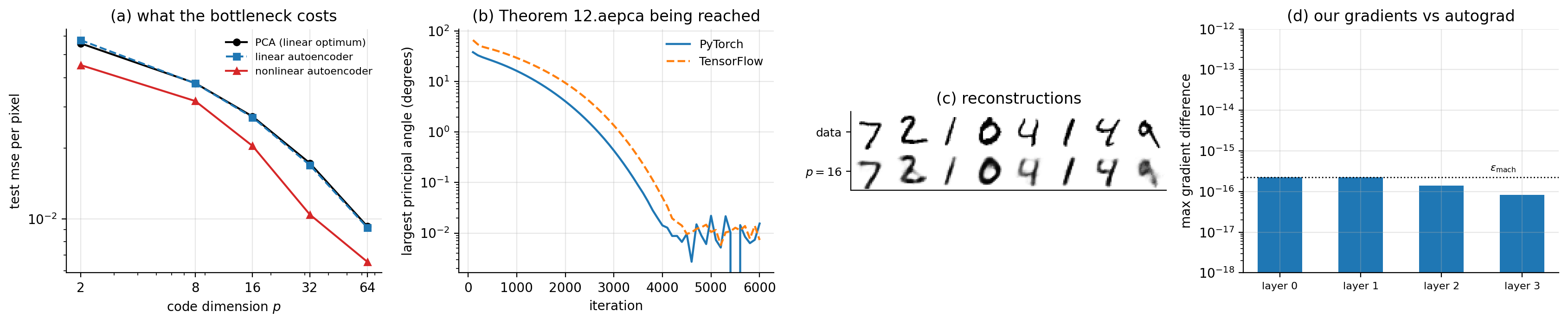
Figure 12.7: (a) Reconstruction error against code dimension on MNIST, Table 12.2: PCA is the floor for any linear map of that rank, the linear autoencoder tracks it, and the nonlinear one beats it by a margin that grows with \(p\). (b) The largest principal angle between the encoder subspace and the span of the top \(p\) eigenvectors, against training iteration, in both frameworks: Theorem 12.5 being reached, not assumed. (c) Test images and their reconstructions at \(p=16\). (d) The largest disagreement between our gradients and each framework’s, against the double-precision unit roundoff.
12.9. Summary and the programs#
An autoencoder approximates the identity through a constrained factorisation, and everything interesting follows from the constraint rather than from the objective.
The linear case is solved completely. Lemma 12.1 reduces the rank-constrained problem to orthogonal projectors, Lemma 12.2 turns reconstruction error into variance not captured, and Theorem 12.4 maximises that variance at the leading eigenvectors. Theorem 12.5 assembles these: the minimum error is the eigenvalue tail \(\sum_{i>p}\lambda_i\) and the learned map is the PCA projector. We measured all of it – the error floor reproduced to six digits, the singular values of \(\bm{W}_e\bm{W}_d\) equal to three ones and five zeros to machine precision, the subspaces agreeing to a fifth of a degree.
Proposition 12.7 is the caveat to carry away. The factorisation is invariant under \(\bm{W}_e\to\bm{W}_e\bm{M}\), \(\bm{W}_d\to\bm{M}^{-1}\bm{W}_d\), so the autoencoder identifies the principal subspace and not the principal directions. Measured: \(\|\bm{W}_e-\bm{U}_p\|_F=1.87\), while the distance from \(\bm{W}_e\) to the span of \(\bm{U}_p\) is \(2.5\times10^{-3}\). If the directions matter, use PCA.
Proposition 12.6 is what turns the theorem into a statement about training. The objective is not convex, but its only non-global critical points are saddles – projections onto the wrong set of eigenvectors, each with an explicit direction of descent – so a first-order method has nowhere bad to stop. Section Does Adam find the principal subspace? confirms the whole chain in one run: Adam reaches the principal subspace to \(0.015\) degrees and the Eckart-Young floor to eight decimals, while missing the principal basis by \(1.34\) per entry.
Nonlinearity buys curvature, at the cost of every guarantee. On a helix in \(\mathbb{R}^{3}\) a one-dimensional nonlinear code beat a two-dimensional linear one, \(0.201\) against \(0.332\), and at equal \(p\) the margin was a factor of four to fifty. On MNIST, Table 12.2, the nonlinear autoencoder beat the exact linear floor at every code dimension and in both frameworks, with the gain largest in the middle of the range rather than at either end. But Figure 12.5(c) showed the reconstruction to be excellent while the code was a poor coordinate, saturating and jumping. Equation (12.2) scores \(\hat{\bm{x}}\) and never mentions \(\bm{z}\), so a good representation is something one must ask for explicitly – by denoising, sparsity, contraction, or by moving to a probabilistic model.
The regularisers were measured too, and one of them broke. Proposition 12.8 shows that denoising at noise level \(\sigma\) is contraction at strength \(\sigma^{2}\) to second order, and the measurements degrade accordingly and gently. The \(\ell_1\) penalty does not: at \(\lambda=0.01\) it halves the number of active code units for a two-thirds rise in error, and at \(\lambda=0.1\) it drives every unit to exactly zero and the model to predicting the mean image. With a ReLU code that collapse is absorbing, and one order of magnitude in \(\lambda\) separates useful from fatal.
The programs are in the directory
doc/BookML/BookPrograms/chapter12_autoencoders.
Every listing above appears there as a numbered file, and three modules run start to finish and reproduce the numbers quoted in the text:
ae.py– the forward and backward passes, Adam, the encode helper, andpcafor comparison.verify_ae.py– the gradient checks of Section Verifying the theorem and the linear-autoencoder-versus-PCA comparison, including the principal angles and the singular values of \(\bm{W}_e\bm{W}_d\).cross_check_ae.py– the three-way comparison of Section PyTorch and TensorFlow.ae_torch.pyandae_tf.py– the principal-subspace test of Section Does Adam find the principal subspace?, the MNIST bottleneck sweep of Table 12.2, and the regularised variants of Section The regularised variants, measured.mnist_data.py– a loader that reads MNIST from a local.npz, so that the programs run without network access.run_nonlinear.py– the helix experiment of Table 12.1.
The figures are generated by ch12_figures.py in
doc/BookML/BookFigures; neither is drawn by hand.
12.10. Exercises#
12.10.1. Warm-up exercises#
The rank factorisation. Show that every \(\bm{A}\in\mathbb{R}^{d\times d}\) with \(\operatorname{rank}(\bm{A})\le p\) can be written as \(\bm{W}_e\bm{W}_d\) with \(\bm{W}_e\in\mathbb{R}^{d\times p}\) and \(\bm{W}_d\in\mathbb{R}^{p\times d}\). This is the step that turns Eq. (12.8) into a statement about ranks rather than about networks.
Projection is optimal. Prove directly that for a subspace \(\mathcal{M}\) and a point \(\bm{x}\), the minimiser of \(\|\bm{x}-\bm{m}\|_2\) over \(\bm{m}\in\mathcal{M}\) is the orthogonal projection, and that the residual is orthogonal to \(\mathcal{M}\). Where exactly is this used in Lemma 12.1?
Trace identities. Verify each step of Lemma 12.2, stating which property of the trace or of \(\bm{P}\) you use at each equality. Then show that \(\operatorname{Tr}(\bm{S})=\sum_i\lambda_i\) for symmetric \(\bm{S}\).
Ky Fan by hand. For \(d=3\), \(p=2\) and \(\bm{\Lambda}=\operatorname{diag}(5,3,1)\), verify Theorem 12.4 by direct computation, and exhibit two different \(\bm{B}\) attaining the maximum. What is the set of all maximisers?
The non-uniqueness. Train a linear autoencoder twice from different seeds and compare (a) the reconstruction errors, (b) the products \(\bm{W}_e\bm{W}_d\), (c) the individual matrices \(\bm{W}_e\). Which two agree and which does not, and why? Then find the matrix \(\bm{M}\) of Proposition 12.7 relating the two runs and check that \(\bm{W}_e^{(1)}\bm{M}\approx\bm{W}_e^{(2)}\).
Overcomplete. Build an autoencoder with \(p>d\) and no regularisation, and confirm that it drives the reconstruction error to zero while learning nothing. Exhibit the weights that achieve this exactly. Then add each of the three regularisers of Section Regularised autoencoders and report what changes.
The landscape. (a) Derive the two stationarity conditions used in the proof of Proposition 12.6 and show they force \(\bm{\Pi}\) to commute with \(\bm{S}\). (b) For \(d=3\), \(p=1\) and \(\lambda=(3,2,1)\), list all three critical projectors, give their objective values, and exhibit the descent direction at each of the two that are not optimal. (c) What goes wrong with the proposition if \(\lambda_p=\lambda_{p+1}\)?
Principal angles. (a) Show that the largest principal angle between two \(p\)-dimensional subspaces is zero if and only if they coincide, and that it equals \(\arccos\sigma_{\min}(\bm{Q}_1^{\mathsf{T}}\bm{Q}_2)\). (b) Show \(\|\bm{\Pi}_1-\bm{\Pi}_2\|_F=\sqrt{2}\,\|\sin\bm{\Theta}\|_F\) for the vector of principal angles \(\bm{\Theta}\), and check the identity against the numbers quoted in Section Does Adam find the principal subspace?. (c) Why is the principal angle, rather than \(\|\bm{W}_e-\bm{U}_p\|\), the right way to compare two runs?
Denoising and contraction. (a) Derive Eq. (12.21), being explicit about where \(\mathbb{E}[\bm{\xi}]=\bm{0}\) and \(\mathbb{E}[\bm{\xi}\bm{\xi}^{\mathsf{T}}]=\bm{I}\) are used. (b) Repeat for masking noise, where each coordinate is zeroed independently with probability \(q\), and identify the penalty that appears. (c) Verify Eq. (12.21) numerically on a trained autoencoder by computing both sides at several \(\sigma\) and confirming the \(\sigma^{2}\) slope.
The sparse collapse. Reproduce the last row of Section The regularised variants, measured. (a) Show that with a ReLU code the all-zero state is a fixed point of the \(\ell_1\)-penalised gradient, so the collapse cannot undo itself. (b) Find the largest \(\lambda\) that still leaves the code alive, to within a factor of two. (c) Replace ReLU by \(\tanh\) or by a soft-thresholding activation and report whether the collapse survives.
Beating PCA. Reproduce Table 12.2 and extend it. (a) At \(p=2\) the linear autoencoder is above the exact floor. Train it longer and report how many epochs are needed to reach the floor to three digits. (b) The gain column is not monotonic. Test the explanation offered in Section What the bottleneck costs, and what the nonlinearity buys by widening the hidden layers and repeating. (c) Add a convolutional autoencoder using Chapter 10 and put it in the same table. Does the convolutional prior help at fixed \(p\)?
12.10.2. Project-style exercise: autoencoders and PCA#
Part a: the machinery. Implement the autoencoder forward and backward passes and verify every gradient against central differences for at least three architectures, including a purely linear one. You will find parameters whose gradient is exactly zero; explain which and why, and make your checker handle them correctly.
Part b: the theorem. Reproduce Section Verifying the theorem on data of your own construction. Confirm Eq. (12.14) to as many digits as your optimiser will give; measure the principal angles; and confirm that the singular values of \(\bm{W}_e\bm{W}_d\) are \(p\) ones and \(d-p\) zeros. Then break the assumption: make \(\lambda_p=\lambda_{p+1}\) exactly and report what happens to part (iii) of the theorem.
Part c: how the floor is approached. Study the convergence of the linear autoencoder to \(\sum_{i>p}\lambda_i\) as a function of the learning rate, the initialisation scale, and the eigenvalue gap \(\lambda_p-\lambda_{p+1}\). Saddle points are known to exist in this landscape corresponding to subsets of eigenvectors other than the leading ones; can you find one, and how long does the optimiser linger there?
Part d: curvature. Reproduce Table 12.1, then vary the curvature of the manifold continuously – for instance by interpolating between a straight line and a helix – and plot the PCA and autoencoder errors against the curvature. At what point does the nonlinear model start to pay for itself?
Part e: representation, not reconstruction. Reproduce Figure 12.5(c) and quantify how badly the code parameterises the curve, for instance by the Spearman correlation between \(z\) and \(t\). Then try to fix it: a wider bottleneck, a different activation, a contractive penalty, more training. Report which of these help and which merely lower the reconstruction error while leaving the code as bad as before. This is the central lesson of the chapter and it deserves evidence.
Part f: the regularisers. Implement the denoising, sparse and contractive objectives of Eqs. (12.17)–(12.20). For the contractive case you will need \(\|\bm{J}_f\|_F^{2}\); obtain it by automatic differentiation and verify it against finite differences. Compare the three on an overcomplete architecture where the bottleneck cannot help.
Part g: convolutional and recurrent. Build a convolutional autoencoder from your Chapter 10 code and a recurrent one from your Chapter 11 code, on the same data. Check the decoder’s output sizes against Proposition 10.4 before training. Compare all three architectures at matched parameter counts and say which inductive bias the data actually reward.
Part h: probabilistic. Implement PPCA, Eq. (12.22), by maximum likelihood, and verify Eq. (12.24) numerically. Use the likelihood to select \(p\) on data where you know the true latent dimension, and compare against choosing \(p\) by the reconstruction-error elbow. Which is more reliable, and does either recover the truth?