
4. Chapter 4: Optimization#
Almost every problem in machine learning begins with a data set \(\bm{X}\), a model \(g(\bm{\theta})\) depending on parameters \(\bm{\theta}\), and a cost function \(C(\bm{X},g(\bm{\theta}))\) measuring how badly the model explains the data. The model is fitted by finding the \(\bm{\theta}\) that minimises the cost. In Chapter 3 we were fortunate: the cost was quadratic, its gradient vanished at a point we could write down, and the minimisation reduced to a linear system. That good fortune does not survive contact with logistic regression, and it certainly does not survive neural networks. For everything that follows in this book we must find minima numerically.
This chapter builds the tools. We begin with the question of when a minimum is worth looking for at all – convexity – and with Newton’s method, which is the ideal we shall spend the rest of the chapter approximating cheaply. We then develop gradient descent, using linear regression as a test bed precisely because we already know the answer, and we identify exactly what makes plain gradient descent slow: the conditioning of the Hessian, a quantity we have already met twice, in Section Vector and matrix norms as a numerical diagnosis and in Section Statistical properties of the least-squares estimator as a statistical one. Everything after that – momentum, stochastic gradients, AdaGrad, RMSProp and Adam – is an attempt to defeat that one number without paying the cost of computing the Hessian.
The reader who wants a single organising idea should hold on to this: gradient descent takes the same step in every direction, but the cost function does not curve equally in every direction, and the whole art lies in fixing that mismatch.
4.1. Convexity#
Ideally we want our cost function to be convex, and it is worth stating precisely what that buys us.
We first need convex sets. A set \(C\subset\mathbb{R}^{n}\) is convex if, for all \(\bm{x}\) and \(\bm{y}\) in \(C\) and all \(t\in(0,1)\), the point \((1-t)\bm{x}+t\bm{y}\) also belongs to \(C\); geometrically, every point on the line segment joining two points of \(C\) lies in \(C\). The convex subsets of \(\mathbb{R}\) are the intervals; examples in \(\mathbb{R}^{2}\) include the regular polygons and the discs.
Convex functions. Let \(X\subset\mathbb{R}^{n}\) be a convex set and \(f:X\rightarrow\mathbb{R}\) continuous. Then \(f\) is convex if
for all \(\bm{x}_1,\bm{x}_2\in X\) and all \(t\in[0,1]\). Replacing \(\le\) by a strict inequality, with \(\bm{x}_1\neq\bm{x}_2\) and \(t\in(0,1)\), defines a strictly convex function. For a function of one variable the condition says that the chord joining \(f(x_1)\) and \(f(x_2)\) lies above the graph on the whole interval \([x_1,x_2]\).
First-order condition. Suppose \(f\) is differentiable. Then \(f\) is convex if and only if its domain \(D_f\) is convex and
for all \(\bm{x},\bm{y}\in D_f\). In words: the first-order Taylor expansion at any point is a global underestimator of the function. Drawing the tangent to \(f(x)=x^{2}+1\) at any point and observing that it lies everywhere below the parabola is enough to make the statement believable.
Second-order condition. If \(f\) is twice differentiable, so that the Hessian exists everywhere, then \(f\) is convex if and only if \(D_f\) is convex and the Hessian is positive semi-definite at every point of \(D_f\). For one variable this reduces to \(f''(x)\ge0\): non-negative curvature everywhere. This condition is the useful one in practice, because it gives a procedure rather than a definition. Proofs of both conditions may be found in Boyd and Vandenberghe [boyd2004].
Why we care. The result that matters is the following.
Any stationary point of a convex function is a global minimum
Let \(f\) be convex and differentiable. Then any \(\bm{x}^{*}\) satisfying \(\nabla f(\bm{x}^{*})=\bm{0}\) minimises \(f\) globally.
The proof is one line from Eq. (4.2): setting \(\bm{x}=\bm{x}^{*}\) makes the gradient term vanish, leaving \(f(\bm{y})\ge f(\bm{x}^{*})\) for every \(\bm{y}\). For a convex cost function, therefore, we need only find a point where the gradient vanishes and we are done – there are no local minima to be trapped in and no saddle points to be delayed by.
We have already used this twice. In Section The Hessian matrix we showed that the least-squares Hessian is \(\bm{H}=\bm{X}^{T}\bm{X}\), positive semi-definite because \(\bm{z}^{T}\bm{X}^{T}\bm{X}\bm{z}=\|\bm{X}\bm{z}\|_2^{2}\ge0\), so the OLS problem is convex and the normal equations (1.39) deliver the global minimum. Adding the Ridge penalty makes the Hessian \(\bm{X}^{T}\bm{X}+\lambda\bm{I}\), positive definite for \(\lambda>0\), so the Ridge problem is strictly convex and its minimum is unique. The Lasso cost of Eq. (3.57) is convex but not differentiable, which is why Section The Lasso needed coordinate descent rather than a gradient.
The bad news is that the cost functions of the later chapters are not convex. A neural network with even one hidden layer has a cost surface with many local minima, and the guarantee above does not apply. We shall nonetheless use methods designed for the convex case, because they work in practice; but it is important to know that when we do so we are relying on empirical good behaviour rather than on a theorem.
4.2. Newton’s method#
Before descending gradients it is worth recalling the method that uses curvature properly, both because it is the standard against which everything else is measured and because its cost is what motivates the alternatives.
Root finding in one dimension. Newton’s method, also called Newton-Raphson, finds a root of \(f\) by extending the tangent line at the current point until it crosses zero. Taylor expanding about a point \(x\) close to the solution \(s\),
and discarding terms beyond the linear one gives \(f(x)+(s-x)f'(x)\approx0\), that is \(s\approx x-f(x)/f'(x)\). As an iteration,
Geometrically \(x_{n+1}\) is where the tangent at \((x_n,f(x_n))\) meets the horizontal axis. Close to a root the convergence is quadratic and extremely fast. Far from one, where the discarded terms matter, the formula can be grossly inaccurate: if an iterate lands near a local extremum, so that \(f'\) nearly vanishes, the method can fail completely. If the derivative is available only numerically, or the function is not smooth, Newton’s method is best avoided.
Several variables. For a system \(f_1(x_1,x_2)=0\), \(f_2(x_1,x_2)=0\), Taylor expansion gives
and collecting the partial derivatives into the Jacobian matrix (1.16),
the update becomes \(\bm{x}^{n+1}=\bm{x}^{n}+\bm{h}^{n}\) with
We must invert the Jacobian, and difficulties arise when it is nearly singular – the conditioning problem of Section Vector and matrix norms again.
Newton’s method for minimisation. Minimising \(C(\bm{\theta})\) means finding a root of \(\nabla C\), so we apply the above with \(\bm{f}=\nabla C\). The Jacobian of the gradient is the Hessian, and the iteration reads
Equation (4.8) is the ideal against which the rest of this chapter should be read. It is what one gets by minimising the second-order Taylor expansion of the cost exactly, and it has two properties no gradient-only method can match: it converges quadratically near the minimum, and it is invariant under linear rescaling of the parameters, so that the conditioning problems which dominate everything below simply do not arise.
Applied to ordinary least squares it is not merely fast but exact. With \(\nabla C=-2\bm{X}^{T}(\bm{y}-\bm{X}\bm{\theta})/n\) from Eq. (1.38) and \(\bm{H}=2\bm{X}^{T}\bm{X}/n\) from Eq. (1.44), a single step from any starting point gives
the exact solution (3.8). This is not a coincidence: for a quadratic cost the second-order Taylor expansion is the function itself, so one Newton step lands on the minimum.
Why we do not simply use it. For \(p\) parameters the Hessian has \(p^{2}\) entries and inverting it costs \(\bigO(p^{3})\) operations by Section LU and Cholesky decompositions. For a linear regression with twenty features this is nothing. For a neural network with \(10^{7}\) parameters the Hessian would need \(10^{14}\) numbers, which cannot be stored, let alone factorised. The entire subject of this chapter is the construction of methods that capture some of the benefit of Eq. (4.8) at a cost linear rather than cubic in \(p\).
4.3. Gradient descent#
The basic idea is that a function \(F(\bm{x})\) decreases fastest, locally, if one moves from \(\bm{x}\) in the direction of the negative gradient \(-\nabla F(\bm{x})\). One can show that for
and for \(\gamma_k\) small enough, \(F(\bm{x}_{k+1})\le F(\bm{x}_k)\): we always move towards smaller function values. Iterating Eq. (4.10) from an initial guess \(\bm{x}_0\) is the method of steepest descent, or simply gradient descent (GD). The parameter \(\gamma_k\) is the step length, or in machine learning the learning rate. We use the symbol \(\gamma\) for it throughout this book, with a subscript when it changes from one iteration to the next.
Ideally the sequence converges to a global minimum. In general we do not know whether a minimum we reach is global or local; but by Section Convexity, if \(F\) is convex the question does not arise. The scheme is conceptually simple and easy to implement. It also has severe limitations.
Limitations. In machine learning we are often faced with non-convex, high-dimensional cost functions with many local minima. Gradient descent is deterministic, so unless the initial guess is good it will descend into whichever local minimum it happens to face, and the result is sensitive to that initial condition. The gradient is a function of all \(p\) parameters and can be expensive to evaluate. And the method is delicate in its dependence on \(\gamma\): we are guaranteed \(F(\bm{x}_{k+1})\le F(\bm{x}_k)\) only for sufficiently small steps, so too large a value produces erratic behaviour or divergence while too small a value converges intolerably slowly. Determining a good \(\gamma\) is the central practical difficulty, and Sections AdaGrad to Adam are devoted to removing the need to do so by hand.
Many of these shortcomings can be alleviated by introducing randomness, which is the subject of Section Stochastic gradient descent.
4.4. Gradient descent for linear regression#
Linear regression is the ideal test case for gradient descent, for three reasons: it has an analytical solution to check against, its gradient can be computed exactly, and its cost function is convex so that convergence is guaranteed for small enough learning rates.
We take the data set used throughout Chapter 3,
with \(n=100\) points, and the design matrix including an intercept column,
The cost function is
Computing \(\partial C/\partial\theta_0\) and \(\partial C/\partial\theta_1\) separately and reassembling,
which is Eq. (1.38) written out coordinate by coordinate. The Hessian is
in agreement with Eq. (1.44), and positive semi-definite, so \(C\) is convex and any stationary point is the global minimum.
The gradient descent iteration is
started from a random \(\bm{\theta}_0\) and stopped when \(\|\nabla_{\bm{\theta}}C\|\le\epsilon\) for some tolerance, say \(10^{-8}\).
import numpy as np

n = 100
rng = np.random.default_rng(2024)
x = 2.0 * rng.random((n, 1))
y = 4.0 + 3.0 * x + rng.normal(size=(n, 1))
X = np.c_[np.ones((n, 1)), x]

# The analytical solution of Chapter 3, for comparison
theta_exact = np.linalg.pinv(X.T @ X) @ X.T @ y
print("analytical:", theta_exact.ravel())

# Gradient descent, Eq. (4.gditeration)
theta = rng.normal(size=(2, 1))
gamma = 0.1
for k in range(1000):
    gradient = (2.0 / n) * X.T @ (X @ theta - y)
    theta -= gamma * gradient
    if np.linalg.norm(gradient) < 1.0e-8:
        break
print(f"gradient descent after {k+1} iterations:", theta.ravel())
With \(\gamma=0.1\) the iteration reproduces the analytical answer to five decimal places within a few hundred steps. With \(\gamma=0.001\), the value used in the lecture notes, a thousand iterations are not nearly enough; with \(\gamma\) too large it diverges. The next section explains exactly where the boundary lies.
4.4.1. Gradient descent for Ridge regression#
The same treatment applies to the Ridge cost of Eq. (3.43). Writing it as
the gradient and Hessian follow from Eqs. (1.25) and (1.28),
Setting the gradient to zero returns the closed form (3.44), as it must. The Hessian is now positive definite for every \(\lambda>0\), so the problem is strictly convex.
import numpy as np

lmbda = 0.001
theta = rng.normal(size=(2, 1))
gamma = 0.1
for k in range(1000):
    gradient = 2.0 * (X.T @ (X @ theta - y) / n + lmbda * theta)
    theta -= gamma * gradient

# Compare with the closed form of Chapter 3
I = np.eye(X.shape[1])
theta_exact = np.linalg.inv(X.T @ X + n * lmbda * I) @ X.T @ y
print("gradient descent:", theta.ravel())
print("closed form:     ", theta_exact.ravel())
Note the factor \(n\) in the closed form. Our cost (4.16) carries \(1/n\) on the data term but not on the penalty, whereas Eq. (3.44) was derived with neither; the two agree only if \(\lambda\) is scaled accordingly. This is precisely the class of bookkeeping error warned against in Section Scaling, centring and the intercept, and it is worth tracking carefully whenever a penalised gradient is implemented.
4.5. The learning rate and the condition number#
We can now answer the question of how large \(\gamma\) may be, and in doing so identify the quantity that governs everything in the rest of this chapter.
Consider a quadratic cost with symmetric positive definite Hessian \(\bm{H}\), which by Eq. (4.14) is the case for least squares. Write the error at step \(k\) as \(\bm{e}_k=\bm{\theta}_k-\bm{\theta}^{*}\), with \(\bm{\theta}^{*}\) the minimum. Since \(\nabla C(\bm{\theta})=\bm{H}\bm{e}\) for a quadratic, the iteration (4.15) gives
Now diagonalise. By the spectral decomposition (1.54), \(\bm{H}=\bm{Q}\bm{\Lambda}\bm{Q}^{T}\) with orthonormal eigenvectors and eigenvalues \(\lambda_i>0\). Expressing the error in the eigenbasis, \(\tilde{\bm{e}}=\bm{Q}^{T}\bm{e}\), and multiplying Eq. (4.18) from the left by \(\bm{Q}^{T}\),
because \(\bm{Q}^{T}\bm{Q}=\bm{I}\) and \(\bm{Q}^{T}\bm{H}\bm{Q}=\bm{\Lambda}\). The matrix on the right is diagonal, so the recursion decouples completely into \(p\) independent scalar recursions:
Each eigendirection contracts by its own factor \(|1-\gamma\lambda_i|\) at every step, and this single equation contains everything.
Stability.
We can now state and prove the condition on the learning rate.
Theorem 4.1 (Stability of gradient descent on a quadratic)
Let \(\bm{H}\) be symmetric positive definite with eigenvalues \(0<\lambda_{\min}\le\lambda_i\le\lambda_{\max}\). The gradient descent iteration (4.15) with fixed learning rate \(\gamma\) converges to \(\bm{\theta}^{*}\) from every starting point \(\bm{\theta}_0\) if and only if
Equivalently, the spectral radius of the iteration matrix satisfies
Proof
By Eq. (4.19) the \(i\)-th component of the error in the eigenbasis is \(\tilde{e}_{k,i}=(1-\gamma\lambda_i)^{k}\tilde{e}_{0,i}\), a geometric sequence with ratio \(1-\gamma\lambda_i\). It tends to zero for every \(\tilde{e}_{0,i}\) precisely when \(|1-\gamma\lambda_i|<1\). Since \(\lambda_i>0\) we may unpack the absolute value:
Because \(\bm{Q}\) is orthogonal, \(\|\bm{e}_k\|=\|\tilde{\bm{e}}_k\|\), so \(\bm{e}_k\to\bm{0}\) for every \(\bm{e}_0\) if and only if every component converges, that is
since \(2/\lambda_i\) is smallest for the largest eigenvalue. This is Eq. (4.20). For the converse, suppose \(\gamma\ge2/\lambda_{\max}\) and take \(\bm{e}_0\) with a non-zero component along the eigenvector of \(\lambda_{\max}\); that component has \(|1-\gamma\lambda_{\max}|\ge1\) and does not decay, so the iteration fails to converge from this \(\bm{\theta}_0\). Finally, the eigenvalues of \(\bm{I}-\gamma\bm{H}\) are \(1-\gamma\lambda_i\) (the eigenvectors are those of \(\bm{H}\)), so its spectral radius is \(\max_i|1-\gamma\lambda_i|\), and the condition just derived is exactly Eq. (4.21).
The bound is set by the steepest direction, whatever the others are doing: the direction of greatest curvature is the one along which a gradient step changes the parameters most, and it is therefore the first to become unstable. Exceed the bound and the component along that direction grows geometrically; this is the divergence one observes when the learning rate is set too high.
At and beyond the bound. It is worth reading off from Eq. (4.19) exactly what the stiffest mode does as \(\gamma\) increases. Its multiplier is \(1-\gamma\lambda_{\max}\), so for \(0<\gamma<1/\lambda_{\max}\) the mode decays monotonically without changing sign; for \(1/\lambda_{\max}<\gamma<2/\lambda_{\max}\) the multiplier is negative and the mode alternates in sign at every step while its magnitude still decreases – this is the zig-zag across the valley in the centre panel of Figure 4.2; at \(\gamma=2/\lambda_{\max}\) the multiplier is exactly \(-1\) and the mode oscillates forever without decaying; and for \(\gamma>2/\lambda_{\max}\) the multiplier has magnitude greater than one and the mode diverges. The strict inequality in Eq. (4.20) is therefore essential: at the boundary itself nothing blows up, but nothing converges either.
Decrease of the cost. The same calculation shows that, inside the stable range, the cost itself decreases at every step and not only the error. For a quadratic with Hessian \(\bm{H}\) the excess cost is \(C(\bm{\theta})-C(\bm{\theta}^{*})=\tfrac12\bm{e}^{T}\bm{H}\bm{e}\), which in the eigenbasis reads
Every non-zero term shrinks when \((1-\gamma\lambda_i)^{2}<1\), which is the condition of the theorem once more. Hence Eq. (4.20) guarantees a strict reduction of the cost at every iterate that is not already the minimum. (For least squares \(\bm{H}=2\bm{X}^{T}\bm{X}/n\), and one checks directly that \(C(\bm{\theta})-C(\bm{\theta}^{*})=\|\bm{X}\bm{e}\|^{2}/n =\tfrac12\bm{e}^{T}\bm{H}\bm{e}\).)
Beyond quadratics.
Nothing in the argument used that the cost was a quadratic globally. Near a minimum \(\bm{\theta}^{*}\) of any twice differentiable cost, \(\nabla C(\bm{\theta}^{*})=\bm{0}\) and Taylor expansion gives \(\nabla C(\bm{\theta})=\bm{H}^{*}\bm{e}+\mathcal{O}(\|\bm{e}\|^{2})\) with \(\bm{H}^{*}=\nabla^{2}C(\bm{\theta}^{*})\), so the recursion (4.18) describes the local dynamics and the theorem gives the local stability condition, with \(\lambda_{\max}\) the largest eigenvalue of the Hessian at the minimum. A global statement needs a global bound on the curvature. Suppose the gradient is Lipschitz continuous with constant \(L\),
which for a twice differentiable cost means that all Hessian eigenvalues lie in \([-L,L]\) everywhere. Then the descent lemma holds: for any \(\bm{\theta}\) and any step \(\bm{d}\),
To see this, write the change in the cost as an integral along the segment from \(\bm{\theta}\) to \(\bm{\theta}+\bm{d}\) and subtract and add \(\nabla C(\bm{\theta})^{T}\bm{d}\) under the integral sign,
the Cauchy–Schwarz inequality and Eq. (4.23) bound the integrand by \(Lt\|\bm{d}\|^{2}\), and \(\int_0^1 Lt\,dt=L/2\). Taking the gradient step \(\bm{d}=-\gamma\bm{g}_k\) with \(\bm{g}_k=\nabla C(\bm{\theta}_k)\),
so the cost decreases strictly, wherever the gradient is non-zero, whenever
This is the “sufficiently small step” promised in Section Gradient descent, now made quantitative. For a quadratic the Lipschitz constant of the gradient is \(L=\lambda_{\max}(\bm{H})\), and the descent lemma reproduces the stability bound (4.20) exactly.
Qualifications. Four remarks delimit what has been proved. Positive definiteness matters: if \(\bm{H}\) has a negative eigenvalue, the corresponding multiplier \(1-\gamma\lambda_i\) exceeds one for every \(\gamma>0\) and no fixed positive learning rate contracts that direction – gradient descent moves away from a saddle point or a maximum, which is what one wants, but the analysis above no longer describes convergence. If \(\bm{H}\) has zero eigenvalues, the multiplier along the corresponding flat directions is exactly one and the quadratic model predicts no contraction at all; for least squares this is the rank-deficient case of Section Ridge regression through the singular value decomposition, and the remedy is the Ridge penalty discussed below. For a non-quadratic cost the eigenvalues vary with \(\bm{\theta}\): the local bound uses the Hessian at the minimum, whereas a global guarantee needs a Lipschitz constant \(L\) valid over the whole region visited by the iterates, which is typically much larger and makes the permitted step correspondingly smaller. And stochastic gradients, the subject of Section Stochastic gradient descent, add noise to every step, so the deterministic bound is a guide to stability rather than a complete convergence theory.
Speed. Inside the stable range the question becomes how fast the error contracts, and the answer is set by the two extreme eigenvalues. The worst-case contraction factor per step is
because \(|1-\gamma\lambda|\) is largest at one end or the other of the spectrum. For \(\gamma\le1/\lambda_{\max}\) the first term dominates and \(r\) decreases with \(\gamma\); for larger \(\gamma\) the second term \(\gamma\lambda_{\max}-1\) grows. The minimum lies where the two are equal, \(1-\gamma\lambda_{\min}=\gamma\lambda_{\max}-1\), which gives the optimal learning rate \(\gamma^{*}=2/(\lambda_{\max}+\lambda_{\min})\) and the contraction rate
where \(\kappa\) is the condition number of the Hessian in the sense of Eq. (1.77). Since \((\kappa-1)/(\kappa+1)\approx1-2/\kappa\) for large \(\kappa\), the number of iterations needed to reduce the error by a fixed factor is proportional to \(\kappa\): a large condition number produces slow convergence even when the learning rate is perfectly stable and optimally chosen.
Figure 4.1 confirms both statements numerically. The iteration count falls as \(\gamma\) increases, reaches its minimum at the predicted \(\gamma^{*}=2/(\lambda_{\max}+\lambda_{\min})\), rises again, and diverges exactly at \(2/\lambda_{\max}\). There is no margin of safety at the right-hand edge: the transition from the fastest convergence available to outright divergence occupies a factor of two in \(\gamma\).
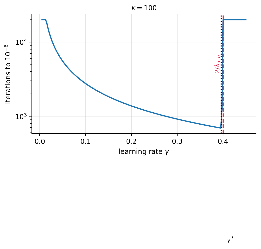
Figure 4.1: Iterations required to reach an error of \(10^{-6}\) against the learning rate, for a quadratic with eigenvalues \(\{0.05,1,5\}\). The optimum lies at \(\gamma^{*}\) and the method diverges beyond \(2/\lambda_{\max}\), as predicted by Eqs. (4.20) and (4.26).
This is the central result of the chapter, and it deserves to be read slowly. Gradient descent is not slow because gradients are a bad idea. It is slow because it applies the same \(\gamma\) to every eigendirection, while stability forces that single \(\gamma\) to be dictated by the steepest direction. In a problem where \(\lambda_{\max}/\lambda_{\min}=1000\), the step that is barely stable along the steep direction is a thousand times too small along the flat one, and the flat direction is where the remaining error lives. The iterates oscillate across the narrow valley while creeping along its floor.
What this means for regression. For least squares \(\bm{H}=2\bm{X}^{T}\bm{X}/n\), so by Eq. (1.118)
and the iteration count scales with the square of the condition number of the design matrix. Three consequences follow, each connecting to earlier chapters.
First, standardising the features is not only the statistical convention of Section Scaling, centring and the intercept but a direct accelerator: it makes the columns of \(\bm{X}\) comparable in scale, reduces \(\kappa\), and thereby reduces the number of iterations. This is the precise sense in which “transform your inputs” is good advice.
Second, Ridge regression improves conditioning as well as variance. By Eq. (4.17) the Hessian becomes \(2(\bm{X}^{T}\bm{X}/n+\lambda\bm{I})\), whose condition number is \((\lambda_{\max}+\lambda)/(\lambda_{\min}+\lambda)\) – smaller than \(\kappa\) for every \(\lambda>0\). Regularisation makes the optimisation easier as well as the estimator better behaved, exactly as anticipated in the notebox of Section Vector and matrix norms.
Third, the conjugate gradient method of Section The conjugate gradient method achieves a rate governed by \(\sqrt{\kappa}\) rather than \(\kappa\), and for a quadratic cost it is strictly superior to gradient descent. It is the right tool for linear regression at scale. Its disadvantage is that it relies on the cost being quadratic and on exact gradients, and it copes badly with the stochastic, non-convex problems of the following chapters – which is why the machine learning literature developed a different set of remedies, to which we now turn.
Figure 4.2 shows what the algebra describes. On an elongated quadratic with \(\kappa=12\), a small learning rate creeps along the valley floor without ever crossing it; a learning rate near the stability bound (4.20) oscillates across the valley while making slow progress along it; and momentum, at the same learning rate, damps the oscillation and accelerates the drift, arriving in a fraction of the steps. The three panels are the whole of this section and the next in pictures.
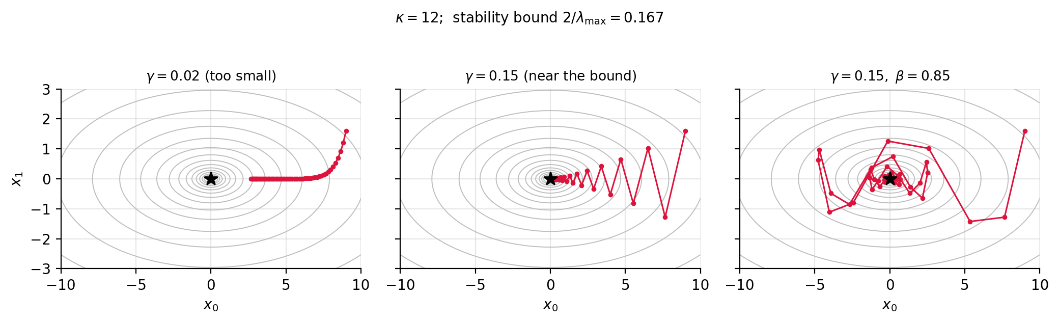
Figure 4.2: Gradient descent on a quadratic with \(\kappa=12\). Left: too small a step. Centre: a step near the stability bound \(2/\lambda_{\max}\), oscillating across the narrow direction. Right: the same step with momentum \(\beta=0.85\), which cancels the oscillation and accumulates along the flat direction.
4.6. Momentum#
The first remedy is to give the iteration a memory of where it has been. Momentum-based gradient descent replaces Eq. (4.10) by
with \(\beta\in[0,1)\) the momentum parameter, typically \(0.9\) (it plays the same role as, and is deliberately given the same letter as, the \(\beta_1\) of the Adam method in Section Adam). The update is no longer the current gradient but an exponentially weighted sum of all gradients seen so far,
with older gradients discounted geometrically. Setting \(\beta=0\) recovers plain gradient descent.
Where the name comes from. The word momentum is not a metaphor. Consider a particle of mass \(m\) moving in the potential \(C(\bm{\theta})\) – the cost function read as a landscape – and subject to a friction force proportional to its velocity, with friction coefficient \(\mu\). Newton’s second law reads
Without friction the particle would roll down the slope, overshoot the bottom and oscillate forever; with friction it loses energy on every swing and settles at a minimum. Now discretise Eq. (4.30) with a time step \(\Delta t\), writing \(\bm{\theta}_k=\bm{\theta}(k\Delta t)\) and replacing the derivatives by finite differences,
Multiplying through by \((\Delta t)^{2}\) and collecting the terms in \(\bm{\theta}_{k+1}\) on the left,
so that the position update is
With \(\bm{v}_{k+1}=\bm{\theta}_k-\bm{\theta}_{k+1}\) this is exactly Eq. (4.28): the new displacement is \(\beta\) times the old one plus \(\gamma\) times the gradient. The momentum parameter is the fraction of its velocity the particle keeps from one step to the next, and the learning rate is the squared time step divided by the effective mass. (Many texts and the slides of this course write the same iteration as \(\bm{v}_{k}=\beta(\bm{\theta}_k-\bm{\theta}_{k-1})-\gamma\nabla C(\bm{\theta}_k)\), \(\bm{\theta}_{k+1}=\bm{\theta}_k+\bm{v}_k\); that is Eq. (4.28) with the sign of \(\bm{v}\) reversed, and nothing else changes.)
The two limits of Eq. (4.31) are instructive. When friction dominates, \(\mu\Delta t\gg m\), we have \(\beta\to0\) and \(\gamma\to\Delta t/\mu\): the particle has no inertia, its velocity is proportional to the force, and the iteration is plain gradient descent – a massless bead sliding through treacle. When friction is negligible, \(\mu\Delta t\ll m\), we have \(\beta\to1\) and \(\gamma\to(\Delta t)^{2}/m\): energy is conserved, the particle never settles, and the iteration rings across the valley indefinitely. This is the frictionless “ball” of the example below, where \(\beta=0.9\) overshoots the global minimum. Between the two, \(1-\beta=\mu\Delta t/(m+\mu\Delta t)\) measures how much energy is dissipated per step. The gain \(1/(1-\beta)\) that we shall meet in Eq. (4.32) below is the terminal velocity of the particle: under a constant force \(\bm{g}\) the steady displacement per step is \(\gamma\bm{g}/(1-\beta)=(\Delta t/\mu)\, \bm{g}\), that is, the velocity \(\bm{g}/\mu\) at which friction exactly balances the force, independent of the mass. What a heavier ball buys is not a higher terminal velocity but a longer memory: it takes about \(1/(1-\beta)\) steps to forget a gradient, which is what averages out the sign-alternating gradients of a steep direction.
The method was introduced under the name heavy-ball method by Polyak [polyak1964], who also derived the rate quoted below; the reading as a discretised equation of motion, and the limits above, follow Qian [qian1999].
Why it works. Return to the decoupled recursion (4.19). Along an eigendirection with eigenvalue \(\lambda_i\), the gradient is \(\lambda_i\tilde{e}_i\) and the momentum iteration becomes a two-term recurrence in \(\tilde{e}\) rather than a one-term one. Its behaviour splits into two regimes, and the split is exactly what we want.
In a flat direction, \(\gamma\lambda_i\ll1\), successive gradients point the same way and Eq. (4.29) adds them up. A constant gradient \(g\) accumulates to
so the effective step is multiplied by \(1/(1-\beta)\) – a factor of ten for \(\beta=0.9\). The method accelerates precisely where plain gradient descent crawls.
In a steep direction, the iterate overshoots and the gradient reverses sign at every step. Successive terms in Eq. (4.29) then alternate in sign and largely cancel, so the accumulated step is smaller than the bare gradient. The oscillation across the narrow valley is damped.
Momentum thus amplifies the consistent and cancels the oscillatory, which is the right treatment for the ill-conditioned landscape diagnosed in Section The learning rate and the condition number. Polyak’s analysis of the two-term recurrence [polyak1964] shows that with optimally chosen \(\gamma\) and \(\beta\) the contraction rate improves from Eq. (4.26) to
so the iteration count scales with \(\sqrt{\kappa}\) instead of \(\kappa\). For \(\kappa=10^{4}\) that is a hundredfold reduction. The reader will notice that \(\sqrt{\kappa}\) is also the rate of the conjugate gradient method quoted in Section The conjugate gradient method; this is not a coincidence, since both build their step out of the current gradient and the previous direction. Momentum is, in effect, conjugate gradients with the optimal coefficients replaced by a fixed constant that need not be recomputed and does not require the cost to be quadratic.
A minimal example. The behaviour is easiest to see on \(f(x)=x^{2}\), where the exact answer is known.
Figure 4.3 shows what the improvement from \(\kappa\) to \(\sqrt{\kappa}\) is worth. At \(\kappa=10^{2}\) momentum saves an order of magnitude in iterations; at \(\kappa=10^{4}\), two. Since Eq. (4.27) tells us that the least-squares Hessian has the condition number of the design matrix squared, condition numbers in this range are entirely ordinary, and the saving is not academic.
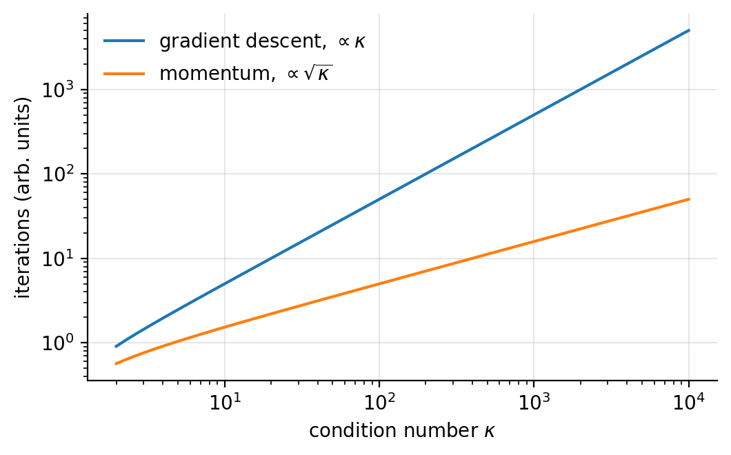
Figure 4.3: Iterations to fixed accuracy against the condition number, for gradient descent and for momentum with optimal parameters, from the rates (4.26) and (4.33).
import numpy as np

def objective(x):
    return x**2.0

def derivative(x):
    return 2.0 * x

def gradient_descent(derivative, bounds, n_iter, step_size, momentum=0.0,
                     rng=None):
    """Gradient descent with optional momentum, Eq. (4.momentum)."""
    rng = np.random.default_rng() if rng is None else rng
    solution = bounds[:, 0] + rng.random(len(bounds)) * (bounds[:, 1] - bounds[:, 0])
    change = 0.0
    solutions, scores = [], []
    for i in range(n_iter):
        gradient = derivative(solution)
        new_change = step_size * gradient + momentum * change
        solution = solution - new_change
        change = new_change
        solutions.append(solution.copy())
        scores.append(objective(solution))
    return solutions, scores


bounds = np.asarray([[-1.0, 1.0]])
rng = np.random.default_rng(4)
plain = gradient_descent(derivative, bounds, 30, 0.1, momentum=0.0,
                         rng=np.random.default_rng(4))
withmom = gradient_descent(derivative, bounds, 30, 0.1, momentum=0.3,
                           rng=np.random.default_rng(4))
print(f"after 30 steps: plain f = {plain[1][-1][0]:.3e}, "
      f"momentum f = {withmom[1][-1][0]:.3e}")
For this one-dimensional problem \(\kappa=1\) and there is nothing to fix, yet momentum still helps by increasing the effective step through Eq. (4.32). The dramatic gains appear when the eigenvalues differ, which is the case for every realistic problem.
Following the steps.
It is worth watching the two iterations step by step on a function simple
enough to be drawn. The function descend below is the whole of
Eq. (4.28), with the gradient passed in as an argument – the
same structure we keep throughout the chapter, so that the analytical
gradient of Section Gradient descent for linear regression and the automatic one of
Section Automatic differentiation are interchangeable.
import numpy as np

def quartic(x):
    """A low-order polynomial with two minima: f(x) = x^4 - 3x^2 + x."""
    return x**4 - 3.0 * x**2 + x

def quartic_grad(x):
    return 4.0 * x**3 - 6.0 * x + 1.0

def descend(grad, x0, gamma, beta=0.0, num_iters=40):
    """Gradient descent with momentum, Eq. (4.momentum); beta = 0 is plain gradient descent.
    Works for a scalar x as well as for a vector theta.  Returns every iterate."""
    x = np.array(x0, dtype=float)
    v = np.zeros_like(x)
    history = [x.copy()]
    for _ in range(num_iters):
        v = beta * v + gamma * grad(x)
        x = x - v
        history.append(x.copy())
    return np.array(history)

for beta in (0.0, 0.7):
    path = descend(quartic_grad, 2.0, gamma=0.05, beta=beta)
    print(f"beta = {beta}: x = {np.round(path[:6], 3)} ... ends at {path[-1]:.4f}, f = {quartic(path[-1]):.4f}")
The quartic \(f(x)=x^{4}-3x^{2}+x\) has a global minimum at \(x=-1.30\) (\(f=-3.51\)), a local one at \(x=1.13\) (\(f=-1.07\)), and a hump at \(x=0.17\) between them. Started at \(x_0=2\) with \(\gamma=0.05\), plain gradient descent walks down into the nearest minimum, \(2\to0.95\to1.01\to1.06\to\dots\to1.131\), and stays there, exactly as Section Gradient descent warned. With \(\beta=0.7\) the velocity built up on the steep slope carries the iterate over the hump, \(2\to0.95\to0.28\to-0.16\to-0.57\to\dots\to-1.302\), into the global minimum: the same code, one extra line, a different answer. This should not be over-read. Momentum knows nothing of the landscape beyond the gradients it has seen; it crossed the hump because the accumulated velocity happened to exceed the barrier, and with \(\beta=0.9\) the “ball” is so frictionless that it overshoots the global minimum, climbs back over the hump and ends in the local basin. Once the cost is not convex, none of the methods of this chapter comes with a guarantee, and Section Convexity is the last time one was available.
The right panel of Fig. 4.4 repeats the exercise on the bowl \(C(\bm{\theta})=\frac12(\theta_1^{2}+10\,\theta_2^{2})\), whose Hessian is \(\mathrm{diag}(1,10)\), so that \(\kappa=10\) and \(2/\lambda_{\max}=0.2\). From \((2,1.4)\), forty steps at \(\gamma=0.04\) creep along the valley floor (356 iterations to reach \(10^{-6}\)); forty steps at \(\gamma=0.18\), just below the bound, zigzag across the steep direction while advancing slowly along the flat one (74 iterations); momentum with \(\beta=0.3\) at the same \(\gamma\) cancels the zigzag and arrives in 39, and the tuned pair \(\gamma=4/(\sqrt{\lambda_{\max}}+\sqrt{\lambda_{\min}})^{2}=0.231\), \(\beta=\bigl((\sqrt\kappa-1)/(\sqrt\kappa+1)\bigr)^{2}=0.27\) that attains the rate (4.33) needs 28. Note that the best \(\beta\) is tied to \(\kappa\): the default \(0.9\) is right for \(\kappa\approx400\) and too much for \(\kappa=10\), where it makes the iterate ring for longer than plain descent takes to converge.
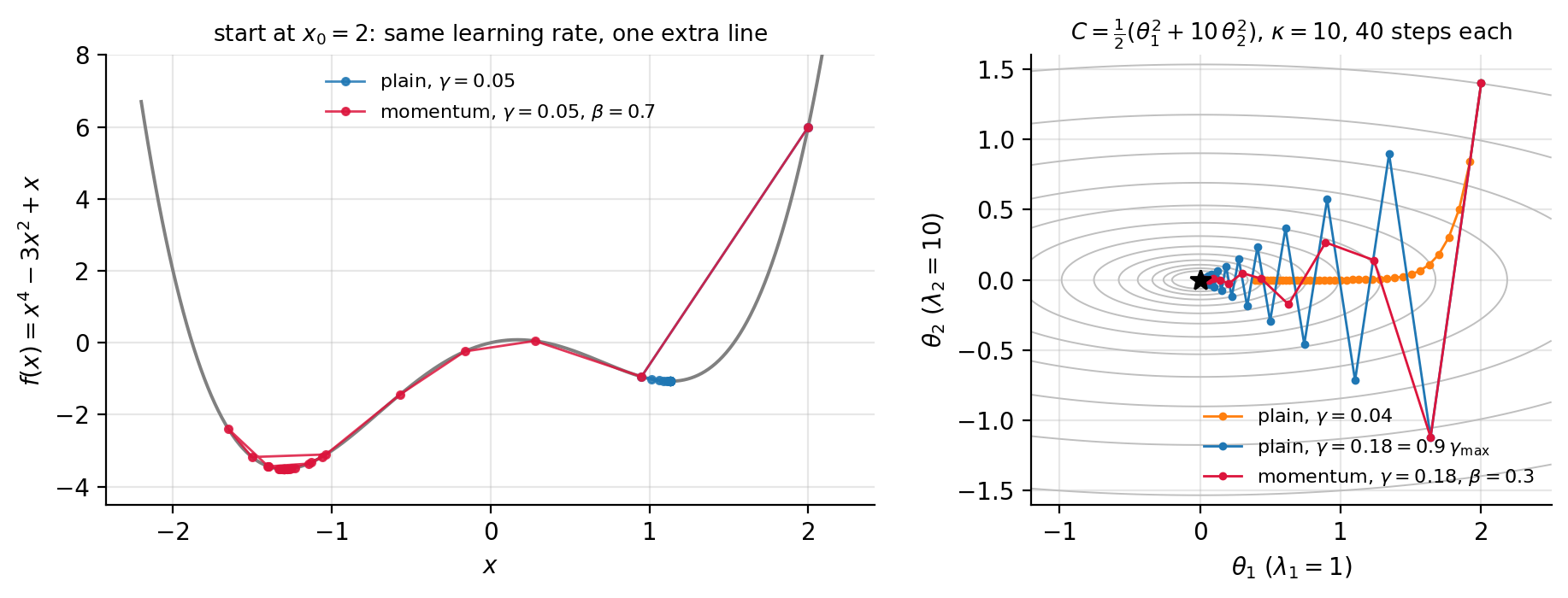
Figure 4.4: Following the steps of gradient descent with and without momentum. Left: the quartic \(f(x)=x^{4}-3x^{2}+x\) from \(x_0=2\) with \(\gamma=0.05\); plain descent stops in the nearer, shallower minimum, momentum with \(\beta=0.7\) carries the iterate over the hump into the global one. Right: forty steps on the bowl \(\frac12(\theta_1^{2}+10\theta_2^{2})\) with \(\kappa=10\), at a small learning rate, at \(0.9\) of the stability bound (4.20), and with momentum \(\beta=0.3\) at the same learning rate.
Machine learning connection
A widely used variant is Nesterov momentum [nesterov1983,sutskever2013], which evaluates the gradient not at \(\bm{\theta}_k\) but at the point the momentum term is about to carry it to, \(\bm{\theta}_k-\beta\bm{v}_k\). The intuition is that of looking ahead before stepping: if the accumulated velocity is about to overshoot, the gradient at the extrapolated point already points backwards and corrects the step early. For convex problems this improves the constant in Eq. (4.33), and in deep learning frameworks it is usually available as a flag on the standard momentum optimiser.
4.7. Stochastic gradient descent#
The second remedy attacks a different problem: cost. Momentum makes each step of gradient descent more effective; stochastic gradient descent makes each step cheaper, by a factor that for the data sets of machine learning runs into the thousands, and accepts a noisy direction as the price. This section makes both halves of that bargain quantitative. We count what an update costs, show that the noisy direction is right on average and by how much it is wrong, work out how far one noisy step can be expected to take us, and then ask the question on which everything turns: how accurate a minimum is worth paying for. The claim that “SGD is faster” is meaningless until an accuracy target and a measure of cost have been named, and most of the confusion about the method comes from leaving one of them out.
4.7.1. The finite-sum problem and the minibatch gradient#
Almost every cost function in machine learning is a sum over data points,
Computing the full gradient therefore costs one pass over the entire data set for a single parameter update. In large-scale applications – the ImageNet challenge has millions of training images – this is extravagant: we spend an enormous computation to obtain one direction, most of whose precision is wasted, since we are going to take another step immediately afterwards.
It is convenient, and from here on we do so, to divide the sum by \(n\) and work with the mean,
as we did for the mean squared error in Eq. (4.12). The minimiser is the same, but the curvature, and with it the stable learning rate of Eq. (4.20), no longer grows with the size of the data set, and the gradient becomes an average – which is what makes it possible to estimate it from a sample.
Stochasticity is introduced by evaluating the gradient on a random subset of the data, called a minibatch. With \(n\) data points and minibatches of size \(M\) there are \(n/M\) minibatches, denoted \(B_k\) with \(k=1,\dots,n/M\). If \(n=10\) and we choose five minibatches, each contains two points: \(B_1=(\bm{x}_1,\bm{x}_2)\) through \(B_5=(\bm{x}_9,\bm{x}_{10})\). Taking \(M=n\) gives a single batch containing everything, which is ordinary gradient descent; taking \(M=1\) gives one point per batch. We approximate
and the update becomes
with a fresh minibatch \(B_t\) for every update. One pass through all the minibatches is called an epoch, and one typically chooses a number of epochs and iterates over the minibatches within each. Dividing by \(M\) rather than summing matters in practice: with the mean, the size of the step does not change when the batch size does, and \(\gamma\) keeps the meaning it had for gradient descent. If a library hands us summed gradients, the learning rate must be divided by \(M\) instead.
Strictly, stochastic gradient descent means using a single example at a time, and the minibatch version should be called minibatch gradient descent; but in practice everyone says SGD and means minibatches, and we shall do the same. The minibatch size is a hyperparameter, but it is seldom tuned by cross-validation: it is usually set by memory constraints, or to a power of two such as \(32\), \(64\) or \(128\), because vectorised operations are fastest at those sizes; Section The batch size, and how to compare fairly returns to this choice with measurements.
Two benefits, and their price. Taking the gradient on a subset has two distinct advantages. It is cheaper: if \(M\ll n\) the gradient costs a fraction of the full one, so we take many more steps for the same computation. And it introduces noise, which decreases the chance of the scheme becoming stuck in a poor local minimum – the deterministic objection raised in Section Gradient descent. A stochastic iterate can be jostled out of a shallow basin in a way a deterministic one cannot.
The corresponding disadvantages are that convergence is erratic rather than monotone, that the iterate does not settle at the minimum but rattles around in a neighbourhood whose size is set by the gradient noise and the learning rate, and that the learning rate must be chosen with more care. The memory picture, on the other hand, is entirely in favour of minibatches: full-batch methods must hold the whole data set, or at least stream it, for every update, whereas SGD needs only the current minibatch. This is what makes training on data sets larger than memory possible at all, and SGD can even begin before the data set is complete, which is the natural setting for streaming data.
4.7.2. What an update costs#
The claim that SGD is ahead per unit of computation can be made exact for the least-squares cost, whose gradient (4.13) is two matrix–vector products: \(\bm{X}\bm{\theta}\) costs \(2np\) floating-point operations (one multiplication and one addition per matrix element), subtracting \(\bm{y}\) costs \(n\), and \(\bm{X}^{T}\bm{r}\) another \(2np\). The minibatch gradient \(\bm{g}_B=\frac{2}{M}\bm{X}_B^{T}(\bm{X}_B\bm{\theta}-\bm{y}_B)\) is the same formula on the \(M\) rows \(\bm{X}_B\in\mathbb{R}^{M\times p}\) of the batch, so
and an epoch of SGD – \(n/M\) updates – costs \(\frac{n}{M}\cdot4Mp=4np\), the same as a single step of gradient descent. This is the comparison to keep in mind: one epoch of minibatch SGD and one update of gradient descent cost the same arithmetic, but during that epoch SGD has changed the parameters \(n/M\) times. Those extra updates help most early in the optimisation, when any reasonable direction makes progress; near the minimum the gradient noise limits what they are worth, as we shall see.
full gradient |
minibatch SGD |
|
|---|---|---|
examples read per update |
\(10^{6}\) |
\(64\) |
operations per update |
\(4\times10^{8}\) |
\(2.56\times10^{4}\) |
updates per epoch |
\(1\) |
\(15\,625\) |
operations per epoch |
\(4\times10^{8}\) |
\(4\times10^{8}\) |
Table 4.1: What one update and one epoch cost for \(n=10^{6}\) observations, \(p=100\) parameters and minibatches of \(M=64\), by the count of Eq. (4.38). If gradient descent needs \(30\) passes over the data to reach a required validation error and SGD needs \(4\), the totals are \(1.2\times10^{10}\) against \(1.6\times10^{9}\) operations, a factor of \(7.5\); the numbers of passes must be measured for the problem at hand, and Section An example where SGD beats gradient descent does so.
Table 4.1 puts numbers on this for a data set of a million points. The arithmetic understates the advantage in wall-clock time, because a minibatch of \(64\) rows stays in the fast cache memory of the processor, while every full gradient drags the entire design matrix through it; and it overstates it for very small batches, for which the overhead of launching an operation exceeds the operation itself. Both effects are measured in Section The batch size, and how to compare fairly.
For comparison, solving the normal equations directly costs about \(np^{2}+p^{3}/3\) flops (forming \(\bm{X}^{T}\bm{X}\), then a Cholesky factorisation, Section LU and Cholesky decompositions), which is \(p/4\) gradient evaluations: for a linear model with modest \(p\) the closed form is the cheapest option of all, and the comparison in this section is between the two iterative methods, which are what remains once the model is a network and no closed form exists.
4.7.3. A worked example: the running mean#
The simplest finite-sum problem shows the whole idea in one line. Let
whose minimiser is the mean \(\hat\theta=\bar a\) of the data. Gradient descent with \(\gamma=1\) finds it in a single update, \(\theta_1=\theta_0-(\theta_0-\bar a)=\bar a\) – but computing that one gradient reads all \(n\) values. SGD with \(M=1\) draws an index \(i_t\) and takes the step
and with the learning rate \(\gamma_t=1/(t+1)\) this is the familiar recursion for a running average: \(\theta_t\) is exactly the mean of the \(t\) values seen so far. By Section The central limit theorem it therefore satisfies
with \(s_a\) the standard deviation of the data. SGD is here nothing but the observation that the mean of a million numbers is known to three digits after looking at a small fraction of them:
import numpy as np

rng = np.random.default_rng(2026)
a = 2.0 + 3.0 * rng.normal(size=1_000_000)        # the data: n = 10^6 numbers
theta = 0.0
for t, i in enumerate(rng.integers(0, len(a), 10_000)):
    gamma = 1.0 / (t + 1)
    theta -= gamma * (theta - a[i])               # SGD step on c_i = (theta - a_i)^2 / 2
    if t + 1 in (100, 1000, 10_000):
        print(f"after {t + 1:6d} samples: theta = {theta:.4f}, error {theta - a.mean():+.4f}, "
              f"s_a/sqrt(t) = {a.std() / np.sqrt(t + 1):.4f}")
print(f"full gradient descent, one step with gamma = 1: theta = {a.mean():.4f}, "
      f"after reading all {len(a)} values")
after    100 samples: theta = 1.6404, error -0.3591, s_a/sqrt(t) = 0.3000
after   1000 samples: theta = 2.0473, error +0.0478, s_a/sqrt(t) = 0.0949
after  10000 samples: theta = 1.9868, error -0.0127, s_a/sqrt(t) = 0.0300
full gradient descent, one step with gamma = 1: theta = 1.9995, after reading all 1000000 values
After one percent of the data the error is \(0.013\), well inside the \(s_a/\sqrt{t}=0.030\) that the central limit theorem allows; over \(2000\) repetitions with \(t=1000\) the errors have mean \(0.005\) and standard deviation \(0.094\), against the predicted \(0.095\). Three features of this toy problem carry over to everything that follows. The stochastic method delivers a useful answer long before the deterministic one has delivered anything. Its error falls as \(1/\sqrt{t}\) in the number of samples and no faster, so that it is a poor way to obtain ten digits. And it needed a decaying learning rate: with a constant \(\gamma\) the recursion (4.40) forgets old samples at the rate it absorbs new ones, and \(\theta_t\) fluctuates forever with variance \(\gamma s_a^{2}/(2-\gamma)\).
4.7.4. The minibatch gradient as an estimator#
Let us make the statement about noise precise. Write \(\bm{g}_i=\nabla c_i(\bm{\theta})\) for the per-example gradients and \(\bm{g}=\nabla C=\frac1n\sum_i\bm{g}_i\) for their mean, and draw the indices \(I_1,\dots,I_M\) of a minibatch independently and uniformly from \(\{1,\dots,n\}\). Conditioned on the current iterate \(\bm{\theta}\) – the only thing the batch is allowed to depend on –
since each index takes each value with probability \(1/n\). The minibatch gradient is an unbiased estimate of the full gradient, whatever \(M\). The conditioning is not a technicality: the argument requires the batch to be chosen without reference to the gradients it contains. Selecting the examples with the largest loss, or reusing the batch on which the previous step did badly, gives a biased direction – sometimes a useful one, but no longer covered by what follows.
For the variance, let \(\bm{\xi}_i=\bm{g}_i-\bm{g}\) be the deviation of example \(i\) from the mean, so that \(\mathbb{E}[\bm{\xi}_I\mid\bm{\theta}]=0\). The \(M\) draws are independent, the cross terms vanish, and
If the batch is instead drawn without replacement, as it is when we shuffle the data and cut the permutation into batches, the elementary theory of sampling from a finite population gives, for component \(j\),
The standard deviation of the estimate falls as \(1/\sqrt{M}\) – not as \(1/M\) – times the finite-population factor \(\sqrt{(n-M)/(n-1)}\), which is one for \(M\ll n\) and vanishes at \(M=n\), where the estimate is the full gradient. Quadrupling the batch size halves the gradient noise at four times the cost per step; that unfavourable exchange rate is why very large batches are not automatically better.
Two things follow. The direction of an SGD step is right on average and wrong in detail, so that an individual update need not decrease \(C\) at all. The amount by which it is wrong depends on \(\bm{\theta}\) through the spread of the per-example gradients – large far from the minimum, and not zero at the minimum, since there the per-example gradients cancel in the sum without vanishing individually. And the noise does not disappear with more iterations, only with a larger \(M\) or a smaller step; the consequences are worked out in Section Learning rate schedules and stopping.
4.7.5. Expected progress in one update, and the rates it implies#
How far does one noisy step take us? Assume, as in Section The learning rate and the condition number, that the gradient is Lipschitz continuous with constant \(L\), so that the descent lemma (4.24) holds, and insert the step \(\bm{d}=-\gamma\bm{g}_B\):
Now take the expectation over the batch, given \(\bm{\theta}_t\). In the linear term unbiasedness, Eq. (4.41), replaces \(\bm{g}_B\) by \(\nabla C\). In the quadratic term we split \(\bm{g}_B=\nabla C+(\bm{g}_B-\nabla C)\); the cross term has expectation zero and the rest is Eq. (4.42), \(\mathbb{E}\|\bm{g}_B\|^{2}=\|\nabla C\|^{2}+\sigma_g^{2}/M\). Collecting terms,
The first two terms are the deterministic result (4.25): on average, a stochastic step makes the progress of a full gradient step. The last term is the price of the noise, and the way the two scale is the whole story of the method. The progress is proportional to \(\gamma\) and to the squared gradient, which is large far from the minimum and vanishes at it; the price is proportional to \(\gamma^{2}/M\) and does not vanish. Far from the minimum the first dominates and SGD advances as if it had the exact gradient, at \(M/n\) of the cost. Close to it the second takes over, and the cost stops decreasing where the two balance – at a level proportional to \(\gamma/M\), which can be lowered only by a smaller learning rate or a larger batch. At the starting point of the example of Section An example where SGD beats gradient descent, with \(M=32\) and \(\gamma=0.02\), the progress term is \(25.6\) and the noise term \(0.74\); none of \(4000\) random minibatches increased the cost. With \(M=1\) and \(\gamma=0.002\), one update in eight did, and the average decrease was still within one percent of the bound.
Rates.
For a strongly convex cost, with all Hessian eigenvalues between \(\mu>0\) and \(L\) and condition number \(\kappa=L/\mu\), the two regimes turn into two convergence rates. Gradient descent at its best learning rate contracts the error by the factor (4.26) per step, and the cost, which is quadratic in the error, by its square,
so reaching an excess cost \(\epsilon\) takes a number of full passes over the data proportional to \(\kappa\) and to the number of digits asked for. For SGD the recursion (4.44) with a learning rate that decays as \(\gamma_t=\beta/(t+t_0)\), \(\beta>1/\mu\), gives instead [bottou2018]
once the memory of the starting point has decayed; without strong convexity the rate degrades to \(\bigO(1/\sqrt{t})\). Per update, then, SGD is far slower than gradient descent: a rate \(1/t\) against a geometric one, the difference between gaining a fixed number of digits per step and needing ten times as many steps for each further digit. But an update of SGD costs \(M/n\) of a full pass, and the product \(Mt\) in Eq. (4.46) is simply the number of examples processed: the accuracy of SGD depends on how much data it has seen, not on how the data were divided into batches, and not on \(n\) at all. The folk statement that “SGD converges faster” conflates these two things. Whether the slow rate at the low price beats the fast rate at the high price depends on how small an \(\epsilon\) we need, and that is a question for statistics.
4.7.6. Which accuracy is worth paying for#
The optimiser works on a finite sample. The minimiser \(\hat{\bm{\theta}}\) of the empirical cost is itself only an estimate of the parameters that minimise the expected cost, with an excess of order
by the variance formula (2.47), and the same scaling \(p/n\) holds for regular parametric models in general. Optimising the empirical cost beyond that accuracy improves the fit to this sample without improving the prediction on the next one, because the next data set would move the minimum by more than that anyway. The target is therefore not \(\epsilon\to0\) but \(\epsilon\sim\epsilon_{\mathrm{stat}}\), and inserting it in the two rates, with \(4np\) flops per step of gradient descent and \(4Mp\) per update of SGD, gives
so that SGD wins by a factor of order \(p\kappa\ln n/M\), which for \(\kappa=10^{2}\), \(p=10^{3}\) and \(M=32\) is several thousand, and grows with the size of the model and the conditioning of the problem. This argument, due to Bottou and Bousquet [bottou2008], is the reason the deep learning frameworks are built around minibatches: for large \(n\) the statistical accuracy that is worth having is reached after a small number of passes over the data, and in that regime SGD is not merely cheaper per step but cheaper to the goal.
The same reasoning says when the conclusion reverses. If what is wanted is a moderate validation error on a large data set, small or medium minibatches usually reach it in a few passes. If what is wanted is the empirical minimiser to many digits – to compare with an analytical result, say, or because a later calculation differentiates through it – the geometric rate of full gradients wins, and so do the variance-reduced methods that combine occasional full gradients with cheap stochastic ones. If the data arrive as a stream, or change while we train, only SGD applies. And if the data set is small, gradient descent, or better the Newton and conjugate gradient methods of Sections Newton’s method and The conjugate gradient method, is simpler and faster. The statement “SGD is faster” always needs an accuracy target and a measure of cost to mean anything.
4.7.7. An example where SGD beats gradient descent#
Figure 4.5 shows the argument at work on a least-squares problem with \(n=10^{5}\) observations and \(p=20\) standardised but strongly correlated features (an autoregressive correlation with coefficient \(0.9\) between neighbouring columns, so that \(\kappa=213\)), unit noise, and \(\bm{\theta}_0=\bm{0}\). The horizontal axis is the number of floating-point operations by Eq. (4.38); the vertical axis is the excess cost \(C(\bm{\theta})-C(\hat{\bm{\theta}})\), and the dotted line is the estimation error \(\sigma^{2}p/n=2\times10^{-4}\) of Eq. (4.47), below which further optimisation is statistically meaningless (the true parameters sit at \(2.6\times10^{-4}\)). Gradient descent at \(\gamma^{*}\) needs \(640\) iterations, \(5\times10^{9}\) flops, to reach that line – the estimate \(t_{\mathrm{GD}}=\frac{\kappa}{4}\ln(C_0/\epsilon)\) of Eq. (4.45) gives \(655\) – and momentum with the tuned \(\gamma\) and \(\beta\) of Eq. (4.33) needs \(81\). SGD with \(M=32\) and the schedule \(\gamma_t=20/(t+1000)\) of Eq. (4.52) first touches it after three to five epochs, depending on the random seed, some \(3\times10^{7}\) flops – two orders of magnitude fewer than gradient descent and one fewer than momentum – and is within a factor of twenty-five of it after a single epoch, before gradient descent has completed its first step. The constant-learning-rate runs make the other point of this section: they are as fast at the start and then level off, at \(10^{-2}\) for \(\gamma=0.02\) and \(3\times10^{-3}\) for \(\gamma=0.005\), the signature of the noise that does not decay.
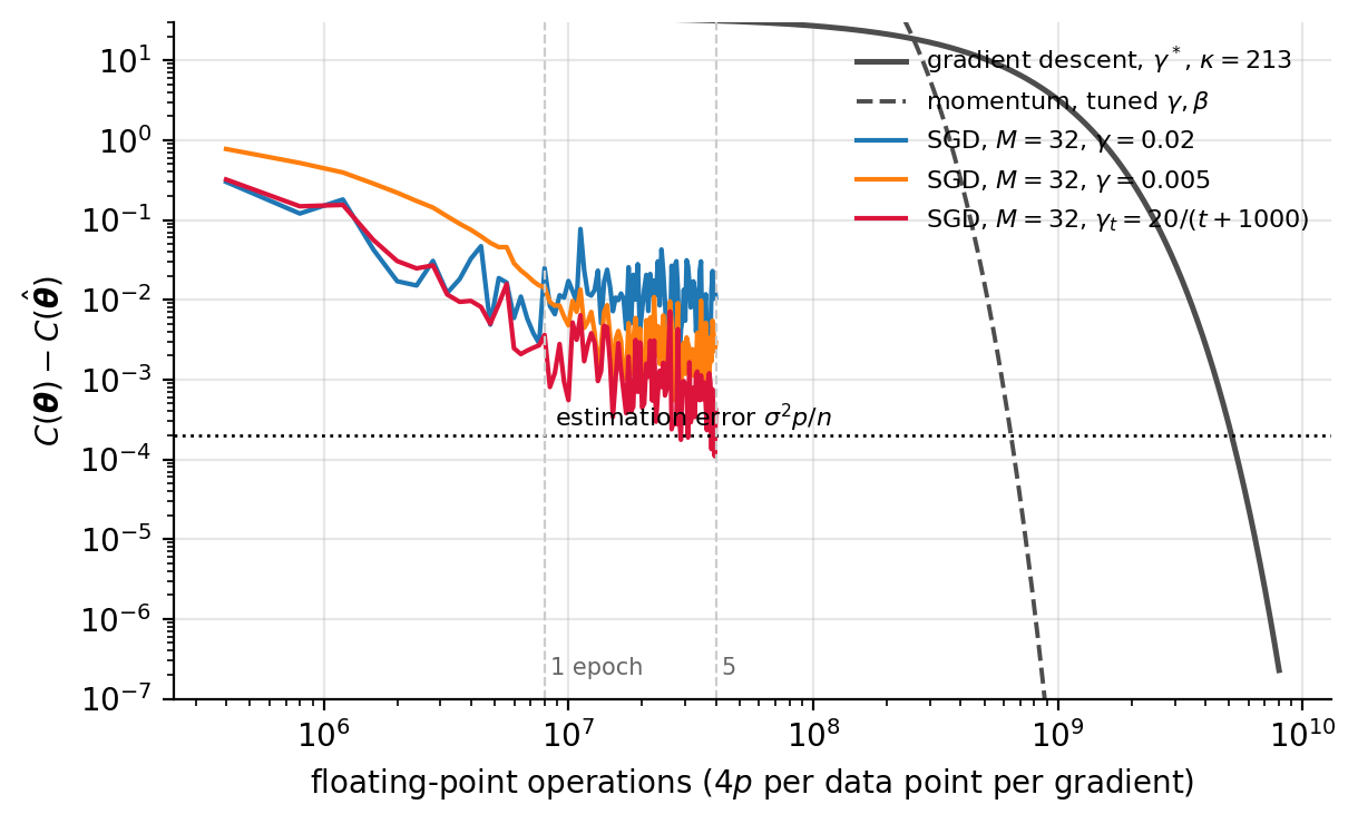
Figure 4.5: Excess cost against floating-point operations on a least-squares problem with \(n=10^{5}\), \(p=20\) and \(\kappa=213\), from \(\bm{\theta}_0=\bm{0}\). Full-batch gradient descent at \(\gamma^{*}\) and momentum with tuned parameters against minibatch SGD (\(M=32\)) at two constant learning rates and with the schedule (4.52). The dotted line is the estimation error \(\sigma^{2}p/n\) of Eq. (4.48); SGD with the schedule is there within five epochs, momentum in \(81\) full gradients and gradient descent in \(640\).
A held-out set of \(20\,000\) points from the same model confirms that the dotted line is the right place to stop. The validation error is \(1.0005\) at the exact minimiser \(\hat{\bm{\theta}}\), \(1.0008\) where gradient descent crosses the line, and between \(1.0006\) and \(1.003\) at the end of the SGD runs of this section: differences in the fourth digit, far below the one percent to which \(20\,000\) points can determine a mean squared error at all. The several hundred further iterations that would take gradient descent from \(10^{-4}\) to \(10^{-10}\) are invisible to any measurement we could make of the quality of the model.
import numpy as np

n, p, rho, sigma = 100_000, 20, 0.9, 1.0
rng = np.random.default_rng(2026)
z = rng.normal(size=(n, p))
X = np.empty_like(z)
X[:, 0] = z[:, 0]
for j in range(1, p):                     # AR(1)-correlated columns: kappa = 213 after standardising
    X[:, j] = rho * X[:, j - 1] + np.sqrt(1 - rho**2) * z[:, j]
X = (X - X.mean(axis=0)) / X.std(axis=0)
theta_true = rng.normal(size=p)
y = X @ theta_true + sigma * rng.normal(size=n)

theta_hat = np.linalg.solve(X.T @ X, X.T @ y)          # np^2 + p^3/3 flops
c_hat = np.mean((X @ theta_hat - y)**2)
excess = lambda th: np.mean((X @ th - y)**2) - c_hat
eigs = np.linalg.eigvalsh((2.0 / n) * X.T @ X)
gamma_star = 2.0 / (eigs.max() + eigs.min())
flops_per_point = 4 * p                                # Eq. (4.flops)

theta = np.zeros(p)                                    # gradient descent: 4np flops per step
for k in range(1, 1001):
    theta -= gamma_star * (2.0 / n) * X.T @ (X @ theta - y)
    if excess(theta) < sigma**2 * p / n:
        print(f"gradient descent reaches sigma^2 p/n after {k} steps = {k * n * flops_per_point:.1e} flops")
        break

M, t, theta = 32, 0, np.zeros(p)                       # SGD: 4Mp flops per update, 4np per epoch
for epoch in range(1, 6):
    for b in np.array_split(rng.permutation(n), n // M):
        t += 1
        gamma = 20.0 / (t + 1000.0)                        # Eq. (4.timedecay)
        theta -= gamma * (2.0 / len(b)) * X[b].T @ (X[b] @ theta - y[b])
    print(f"SGD epoch {epoch}: excess cost {excess(theta):.2e} after {t * M * flops_per_point:.1e} flops")
4.7.8. Learning rate schedules and stopping#
Because the gradient noise does not decay, a constant learning rate leaves the iterate bouncing around the minimum forever. This can be quantified. Take a single eigendirection of a quadratic cost, with curvature \(\lambda\), and write the minibatch gradient as the exact gradient \(\lambda e_t\) plus a noise term \(\xi_t\) of mean zero and variance \(\sigma_g^{2}/M\) by Eq. (4.42), independent from step to step. The error then obeys
the recursion (4.19) driven by noise. Its mean contracts as before, but its second moment obeys \(\mathbb{E}[e_{t+1}^{2}]=(1-\gamma\lambda)^{2}\,\mathbb{E}[e_t^{2}]+\gamma^{2}\sigma_g^{2}/M\), the cross term vanishing because the noise is independent of the current error, and for \(0<\gamma\lambda<2\) it settles at the fixed point
The iterate does not converge; it equilibrates, in a cloud around the minimum whose radius scales as \(\sqrt{\gamma/M}\) – largest along the flat directions, where \(\lambda\) is small – and which no number of further iterations will shrink.
The plateau in the cost. What we observe is not the error along one direction but the excess cost, and for it the result is simpler still. Near the minimum \(C-C^{*}=\frac12\sum_i\lambda_ie_i^{2}\), and in the sum over eigendirections the curvature cancels against the \(1/\lambda_i\) of Eq. (4.50):
with \(\bm{S}\) the covariance matrix of the per-example gradients at the minimum. The plateau is proportional to \(\gamma/M\) and does not depend on the condition number: the flat directions have large clouds, but large clouds in flat directions cost little. For least squares \(\bm{g}_i=2\bm{x}_ir_i\) with \(r_i\) the residual, so that for standardised features \(\mathrm{tr}\,\bm{S}\approx4\sigma^{2}p\) and the plateau is at
The comparison is striking: a constant learning rate reaches the statistical accuracy only if \(\gamma/M\le1/n\). In the example above \(\mathrm{tr}\,\bm{S}=80.2\), and Eq. (4.51) predicts \(1.25\times10^{-2}\) for \(\gamma=0.02\) and \(3.1\times10^{-3}\) for \(\gamma=0.005\) at \(M=32\) – the two levels seen in Fig. 4.5. The right panel of Fig. 4.6 repeats the measurement for seven combinations of \(\gamma\) and \(M\); all but one fall on the line within thirty percent. The exception, \(\gamma=0.05\) with \(M=512\), lies a factor \(1.7\) above it, because there \(\gamma\lambda\) is of order one for the steepest directions and the factor \(2-\gamma\lambda\) of Eq. (4.50) can no longer be replaced by two.
Equation (4.51) says exactly what the remedies are: a smaller \(\gamma\) (at the price of slower progress early on), a larger \(M\) (at the price of \(M\) per step), or a \(\gamma\) that starts large and ends small.
Decaying learning rates. The standard remedy is the last: let \(\gamma\) decay with time. Let \(e=0,1,2,\dots\) index the epoch, let \(m=n/M\) be the number of minibatches, and count updates by \(t=e\cdot m+i\) with \(i=0,\dots,m-1\). A common choice is
with \(t_0,t_1>0\) fixed. The learning rate starts at \(\gamma_0=t_0/t_1\), stays near it for the first \(t_1\) updates – a warm phase in which the iterate moves rapidly towards the right region – and then decays as \(1/t\), shrinking the cloud as it goes. The classical conditions for convergence, due to Robbins and Monro [robbins1951], are
The first ensures that the iterate can still reach the minimum from any starting point; the second that the accumulated noise, which by Eq. (4.49) enters with weight \(\gamma_t^{2}\), is finite. Equation (4.52) satisfies both; a constant satisfies neither. So does the more general polynomial decay
whose smaller exponents decay more gently and are more forgiving of a badly chosen \(t_1\). In a finite run the first condition bites in practice as well as in principle: with \(t_1\) small the learning rate has collapsed after a few hundred updates and the accumulated step \(\sum_t\gamma_t\) over the run is too short to cross an ill-conditioned valley, so the iterate freezes far from the minimum. The cure is to keep the initial rate \(t_0/t_1\) and enlarge both constants, which delays the decay; the schedule in Fig. 4.5 uses \(t_0=20\), \(t_1=1000\). Note also that the schedule counts updates, so that changing the batch size changes how far the learning rate has decayed after one epoch; schedules do not transfer from one \(M\) to another without adjustment.
If the decay is slow compared with the time the iterate needs to equilibrate, the excess cost simply follows the plateau of the current learning rate, \(\gamma_t\,\mathrm{tr}\,\bm{S}/(4M)\). For the schedule (4.52) and \(t\gg t_1\) this is \(t_0\,\sigma^{2}p/(Mt)\), the \(1/(Mt)\) of Eq. (4.46), and measured in epochs \(e=tM/n\) it becomes
after \(e\) epochs the mean excess cost is \(t_0/e\) times the estimation error, whatever the batch size. For the run of Fig. 4.5, averaged over five seeds, the measured values are \(1.3\times10^{-3}\), \(8.0\times10^{-4}\) and \(2.4\times10^{-4}\) after \(3\), \(5\) and \(12\) epochs, against \(1.3\times10^{-3}\), \(7.9\times10^{-4}\) and \(3.3\times10^{-4}\) from the formula. The curve touches the dotted line after three epochs because it fluctuates by a factor of a few around its mean; by Eq. (4.55) the mean arrives there after about \(t_0=20\) epochs – still thirty times sooner than gradient descent.
Averaging the iterates.
There is a second way to remove the noise, which does not slow the iterate down at all: keep the learning rate constant and average the iterates, \(\bar{\bm{\theta}}_T=\frac1T\sum_{t}\bm{\theta}_t\), over the part of the run spent on the plateau. The iterates scatter around the minimum with mean zero, and their average converges to it at the statistically optimal rate, a result due to Polyak and Juditsky [polyak1992]. In the example, five epochs at the constant \(\gamma=0.02\) leave the last iterate at \(1.1\times10^{-2}\), on the plateau of Eq. (4.51); the average of the iterates of epochs three to five has an excess cost of \(2.3\times10^{-6}\), four orders of magnitude lower and a hundred times below the estimation error. The averaged iterate costs one extra vector of storage and one addition per update. For non-convex problems the average can straddle several basins and must be used with care, but exponentially weighted versions of it are common practice in the training of large networks.
A practical SGD loop. The listing below assembles the pieces into the loop one actually writes. Four details deserve attention. The data are shuffled once per epoch and cut into batches, so that every observation is used exactly once per epoch, and the last, smaller batch is kept rather than discarded. The gradient is the mean over the batch, so that the learning rate does not have to change with \(M\). The features are standardised – with the statistics of the training set only – so that no single coordinate dictates the stable learning rate, as discussed in Section The learning rate and the condition number. And the loop stops on the cost of a validation set, not on the gradient.
import numpy as np

def shuffled_batches(n, M, rng):
    """One epoch: every index once, in random order; the last batch may be smaller."""
    idx = rng.permutation(n)
    for k in range(0, n, M):
        yield idx[k:k + M]

def cost(theta, X, y):
    return np.mean((X @ theta - y)**2)

def gradient(theta, X, y):                     # mean over the rows handed in, Eq. (4.meancost)
    return (2.0 / len(y)) * X.T @ (X @ theta - y)

rng = np.random.default_rng(2026)
n, p, rho = 60_000, 20, 0.9
z = rng.normal(size=(n, p)); X = np.empty_like(z); X[:, 0] = z[:, 0]
for j in range(1, p):
    X[:, j] = rho * X[:, j - 1] + np.sqrt(1 - rho**2) * z[:, j]
y = X @ rng.normal(size=p) + rng.normal(size=n)
X_train, y_train, X_val, y_val = X[:50_000], y[:50_000], X[50_000:], y[50_000:]
mean, std = X_train.mean(axis=0), X_train.std(axis=0)      # training set only
X_train, X_val = (X_train - mean) / std, (X_val - mean) / std

M, gamma0, t0, max_epochs, patience = 32, 0.02, 1000.0, 100, 5
theta, t = np.zeros(p), 0
best_val, best_theta, waited = np.inf, theta.copy(), 0
for epoch in range(1, max_epochs + 1):
    for batch in shuffled_batches(len(y_train), M, rng):
        t += 1
        gamma = gamma0 * t0 / (t + t0)                     # Eq. (4.timedecay)
        theta -= gamma * gradient(theta, X_train[batch], y_train[batch])
    val = cost(theta, X_val, y_val)
    if val < best_val - 1e-5:                              # early stopping on the validation cost
        best_val, best_theta, waited = val, theta.copy(), 0
    else:
        waited += 1
    print(f"epoch {epoch:2d}: gamma = {gamma:.1e}, "
          f"training cost {cost(theta, X_train, y_train):.4f}, validation cost {val:.4f}")
    if waited == patience:
        break
theta_ols = np.linalg.lstsq(X_train, y_train, rcond=None)[0]
print(f"stopped after {epoch} epochs; best validation cost {best_val:.4f} "
      f"(least-squares solution: {cost(theta_ols, X_val, y_val):.4f})")
epoch  1: gamma = 7.8e-03, training cost 1.0048, validation cost 1.0239
epoch  2: gamma = 4.8e-03, training cost 1.0024, validation cost 1.0205
epoch  3: gamma = 3.5e-03, training cost 1.0019, validation cost 1.0201
...
epoch  9: gamma = 1.3e-03, training cost 1.0010, validation cost 1.0182
...
epoch 14: gamma = 8.7e-04, training cost 1.0017, validation cost 1.0200
stopped after 14 epochs; best validation cost 1.0182 (least-squares solution: 1.0186)
After three epochs the validation cost is within two parts in a thousand of what the exact least-squares solution achieves, and the best of the fourteen epochs is, by the luck of the noise, marginally below it; the patience of five epochs is what stops the loop from reacting to fluctuations of that size.
When do we stop?. One possibility is to compute the full gradient every few epochs and stop when its norm falls below a threshold. But a vanishing gradient identifies a stationary point, not necessarily a good one, so it is wiser to evaluate the cost at that point, record it, and continue: if the criterion triggers again later, keep whichever \(\bm{\theta}\) gave the lower value. Because the scheme is random by design, repeating the whole computation gives a different answer each time, and taking the best of several runs is a legitimate and common strategy.
In machine learning the more useful criterion is not about the gradient at all. As advised in Section Training error, test error and generalisation, one monitors the cost on a held-out validation set and stops when it begins to rise while the training cost is still falling, as the loop above does. This is early stopping, and it is a regularisation method as much as a termination rule: halting before the variance term of Eq. (2.52) has grown is another way of trading a little bias for a lot of variance, in the same spirit as the Ridge penalty of Section Ridge regression.
4.7.9. The batch size, and how to compare fairly#
The batch size changes the statistics and the use of the hardware at the same time, and the two pull in opposite directions. Table 4.2 lists what is traded.
small batch |
large batch |
|
|---|---|---|
gradient variance |
large |
small, \(\propto1/M\) |
updates per epoch |
many |
few |
hardware efficiency |
poor: overhead dominates |
good, until the processor saturates |
memory |
small |
larger |
late-stage accuracy |
needs decay or averaging |
more stable at a fixed \(\gamma\) |
Table 4.2: What the minibatch size trades. The statistical rows follow from Eqs. (4.42) and (4.51); the hardware rows are measured for our example in Table 4.3.
A simple model of the wall time of one update is
with \(T_{\mathrm{overhead}}\) the fixed cost of launching the operations and \(R(M)\) the rate, in examples per second, at which the hardware processes a batch once it is running. The left panel of Fig. 4.6 shows both for our example, on one core of a laptop; the absolute numbers will differ on another machine, the shape will not. An update with \(M=1\) takes \(5\,\mu\mathrm{s}\) and one with \(M=32\) takes \(7\,\mu\mathrm{s}\): up to a few tens of examples the batch is essentially free, because the time goes into the overhead of the interpreter and of the library calls. The throughput rises from \(2\times10^{5}\) examples per second at \(M=1\) to \(1.5\times10^{7}\) at \(M\approx2000\), where it saturates, and falls again for the full batch of \(10^{5}\) rows, which no longer fits in the cache.
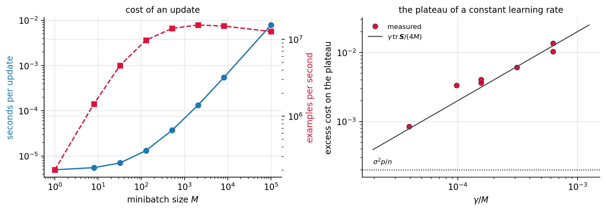
Figure 4.6: Left: measured time per SGD update and throughput in examples per second against the minibatch size, for the least-squares problem of Fig. 4.5; the update is nearly free up to \(M\approx30\), and the throughput saturates near \(M=2000\), the two regimes of Eq. (4.56). Right: the excess cost at which SGD with a constant learning rate levels off, for seven combinations of \(\gamma\) and \(M\), against the prediction \(\gamma\,\mathrm{tr}\,\bm{S}/(4M)\) of Eq. (4.51); the dotted line is the estimation error \(\sigma^{2}p/n\).
Method |
\(\gamma_0\) |
\(t_1\) |
updates |
epochs |
flops |
time (s) |
|---|---|---|---|---|---|---|
gradient descent |
\(0.0885\) |
– |
\(640\) |
\(640\) |
\(5.1\times10^{9}\) |
\(5\) |
SGD, \(M=1\) |
\(0.002\) |
\(10^{4}\) |
\(335\,000\) |
\(3.4\) |
\(2.7\times10^{7}\) |
\(1.7\) |
SGD, \(M=8\) |
\(0.01\) |
\(10^{3}\) |
\(40\,625\) |
\(3.2\) |
\(2.6\times10^{7}\) |
\(0.2\) |
SGD, \(M=32\) |
\(0.02\) |
\(10^{3}\) |
\(9\,370\) |
\(3.0\) |
\(2.4\times10^{7}\) |
\(0.07\) |
SGD, \(M=128\) |
\(0.08\) |
\(300\) |
\(2\,344\) |
\(3.0\) |
\(2.4\times10^{7}\) |
\(0.03\) |
SGD, \(M=512\) |
\(0.08\) |
\(10^{3}\) |
\(1\,124\) |
\(5.8\) |
\(4.6\times10^{7}\) |
\(0.04\) |
Table 4.3: Reaching the estimation error \(\sigma^{2}p/n=2\times10^{-4}\) on the problem of Fig. 4.5: gradient descent at \(\gamma^{*}\) against SGD at five batch sizes, each with the best schedule \(\gamma_t=\gamma_0t_1/(t+t_1)\) of a small grid. Updates, epochs and floating-point operations are medians over five seeds of the first time the excess cost, recorded twenty times per epoch, is below the line; the wall time is the number of updates times the measured time per update and is machine dependent.
Table 4.3 and Fig. 4.7 put the two halves together. Counted in epochs, the batch size hardly matters: from \(M=1\) to \(M=128\) every run is at the line after three passes over the data, as Eq. (4.55) says it should be, and only at \(M=512\), where a pass contains too few updates for the warm phase, does the count rise. Counted in updates the runs differ by a factor of three hundred, and counted in seconds by a factor of sixty, in the opposite order: \(M=1\) wastes the hardware, and the best batch size is the largest one that does not yet cost extra epochs – here \(M\approx128\), near the point where the throughput saturates, and not \(M=1\). Gradient descent, finally, is the fastest of all per update and the slowest by a factor of a hundred and fifty in time.
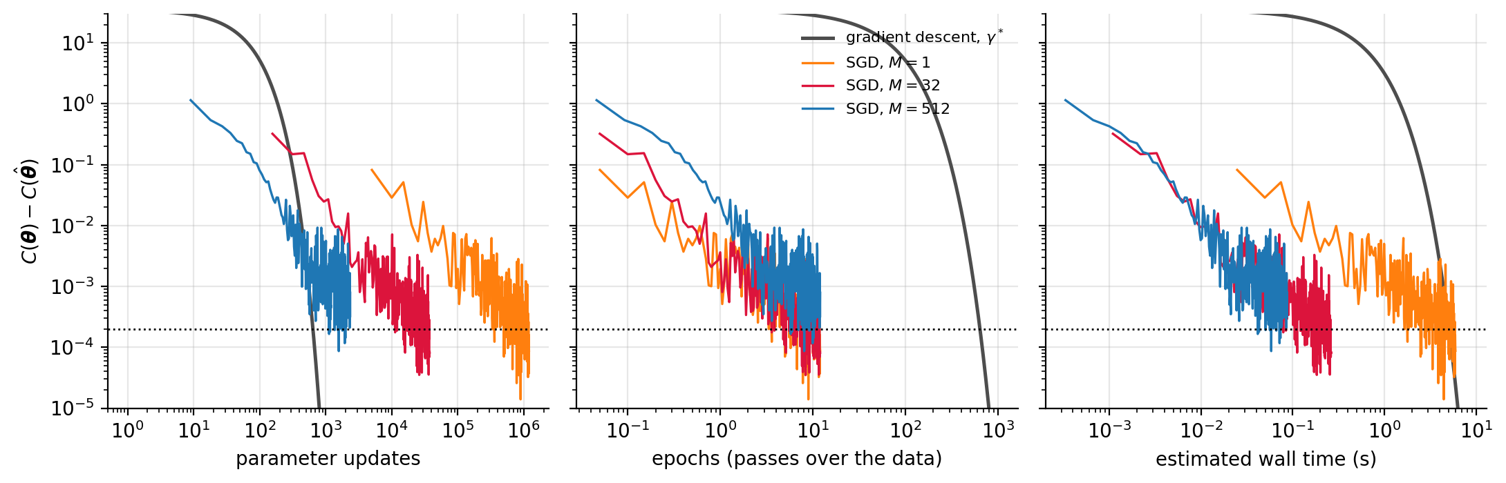
Figure 4.7: The same four runs – gradient descent at \(\gamma^{*}\) and SGD with \(M=1\), \(32\) and \(512\) and the schedules of Table 4.3 – against three horizontal axes. Left: parameter updates, which favours gradient descent. Centre: epochs, that is, the amount of data processed, on which the three SGD runs coincide. Right: estimated wall time, on which the small batch falls behind. The dotted line is the estimation error \(\sigma^{2}p/n\).
Three axes, three stories. Figure 4.7 is a warning as much as a result. A plot of the cost against the number of updates favours whoever has the most expensive update, since gradient descent makes one per epoch; a plot against epochs compares the amount of data processed; a plot against wall time includes memory traffic, parallelism, compilation and communication, and is the one the user of the method cares about. An efficiency claim without a common and stated horizontal axis is incomplete. For a comparison to be fair one should, in addition: use the same training and validation split for all methods; tune the learning rate or the schedule separately for each method, since the best \(\gamma\) of one is rarely the best of another; compare at equal validation performance rather than at an equal number of iterations; and repeat the stochastic runs over several seeds and report the spread, which behind Table 4.3 is up to a factor of \(1.8\) between the luckiest and the unluckiest of five. The exercises ask for this protocol on problems with several condition numbers: ill conditioning slows gradient descent in proportion to \(\kappa\), and it slows SGD as well, through the requirement \(\beta>1/\mu\) behind Eq. (4.46), which is where momentum and the preconditioning of the following sections come in.
When SGD is not the more efficient method. Full gradients can win, and it is as well to know when: when \(n\) is small enough for the whole data set to sit comfortably in fast memory; when the required solution is very accurate; when the per-example gradients have an extremely large variance, so that a minibatch says little about the direction; when large matrix operations use the hardware so much better than small ones that the throughput of Fig. 4.6 outweighs the number of updates; and when the objective permits a cheap sufficient statistic. Least squares is the standard example of the last: forming \(\bm{X}^{T}\bm{X}\) and \(\bm{X}^{T}\bm{y}\) once costs a single pass over the data, after which every gradient costs \(p^{2}\) operations independently of \(n\) – attractive when \(p\ll n\) and the \(p\times p\) matrix fits in memory, though it squares the condition number, Eq. (4.27), and must be weighed against the numerical stability of doing so.
A precise conclusion
SGD is computationally efficient when a useful solution requires only a few passes over the data and each minibatch carries enough information about the direction to make progress. Both conditions hold for the large, noisy, redundant data sets of machine learning, where the accuracy worth having is \(\sigma^{2}p/n\) and not machine precision; neither holds for a small, clean problem that must be solved to many digits. The minibatch gradient is unbiased with variance \(\propto1/M\); a constant learning rate leaves a plateau \(\gamma\,\mathrm{tr}\,\bm{S}/(4M)\) in the cost; decaying rates, iterate averaging and validation-based stopping are what convert cheap noisy updates into useful accuracy; and the efficiency must be reported against examples processed, operations or wall time, at the same validation performance.
4.8. Why adapt the step size at all#
In stochastic gradient descent, with or without momentum, we still have to specify a schedule for the learning rate \(\gamma_t\). Section The learning rate and the condition number showed exactly why this is awkward, and it is worth restating the diagnosis in the form that motivates what follows.
A fixed \(\gamma\) is hard to get right. If it is too large the updates overshoot and the iteration oscillates or diverges, by Eq. (4.20); if it is too small, convergence takes forever, by Eq. (4.26). But the deeper problem is not the choice of a number: it is that no single number is right for all directions. The stability bound is set by \(\lambda_{\max}\) and the convergence rate by \(\lambda_{\min}\), and when these differ by orders of magnitude the step which is barely safe along the steep direction is hopelessly small along the flat one. Steep coordinates need small steps; flat coordinates could take large ones. In high-dimensional problems with features of varying scale, or with sparse features that are active only occasionally, the mismatch is severe.
Ideally our algorithm would keep track of curvature and take large steps in shallow directions and small steps in steep ones. That is precisely what Newton’s method (4.8) does, by normalising the gradient with \(\bm{H}^{-1}\); and the invariance this buys is why Section Newton’s method called it the ideal. The trouble, again, is the \(\bigO(p^{3})\) cost of forming and inverting the Hessian, which is out of the question for large models.
The methods of this section are a compromise. They approximate the curvature information in \(\bm{H}\) using only quantities already available – the gradients themselves – and they restrict the approximation to a diagonal matrix, so that inverting it costs \(\bigO(p)\) rather than \(\bigO(p^{3})\). Instead of tracking the gradient alone, they track the second moment of the gradient. The family includes AdaGrad, AdaDelta, RMSProp and Adam, and we develop the three named in the chapter title.
The idea in one paragraph. Suppose we replace the scalar \(\gamma\) by a diagonal matrix, so that coordinate \(j\) has its own step size \(\gamma/\sqrt{r_j}\). What should \(r_j\) be? Near a minimum the gradient along direction \(j\) behaves as \(g_j\approx\lambda_j e_j\), so a large curvature \(\lambda_j\) produces large gradients and a small curvature produces small ones. The typical magnitude of the gradient in a direction is a proxy for the curvature in that direction. Averaging \(g_j^{2}\) over recent steps therefore estimates something like \(\lambda_j^{2}\) without ever forming a second derivative, and dividing by its square root approximates the \(\bm{H}^{-1/2}\) scaling. This is the entire principle behind AdaGrad, RMSProp and Adam; the three differ only in how the average is taken.
The idea made precise: diagonal preconditioning. All three methods are instances of the preconditioned iteration
with Newton’s method the case \(\bm{D}=\bm{H}\) and gradient descent the case \(\bm{D}=\bm{I}\). For a quadratic cost the error recursion becomes \(\bm{e}_{t+1}=(\bm{I}-\gamma\bm{D}^{-1}\bm{H})\bm{e}_t\), so what governs stability and speed is no longer the spectrum of \(\bm{H}\) but that of \(\bm{D}^{-1}\bm{H}\). When \(\bm{H}\) is diagonal and \(\bm{D}\) tracks its diagonal, \(\bm{D}^{-1}\bm{H}=\bm{I}\): every direction contracts at the same rate, the condition number has been reduced to one, and the iteration count no longer depends on \(\kappa\) at all. When \(\bm{H}\) has off-diagonal entries, no diagonal \(\bm{D}\) can achieve this; the best a diagonal preconditioner can do is bounded by how far \(\bm{H}\) is from diagonal, and a valley that runs at \(45^\circ\) to the axes, with the two coordinates equally scaled, is not improved at all. Figure 4.8 shows both cases on the bowl with eigenvalues \(1\) and \(100\): on the axis-aligned bowl the adaptive methods set off diagonally, both coordinates moving at about \(\gamma\) per step, and reach \(\|\bm{\theta}\|<10^{-4}\) in \(297\) (AdaGrad), \(52\) (RMSProp) and \(151\) (Adam) iterations against \(546\) for gradient descent at \(0.9\cdot2/\lambda_{\max}\) and \(162\) for momentum; on the same bowl rotated by \(45^\circ\) gradient descent and momentum are unchanged, because Eq. (4.19) depends only on the eigenvalues, while AdaGrad and RMSProp no longer reach \(10^{-4}\) in \(5000\) iterations and Adam needs \(635\). The adaptive methods see the diagonal of the Hessian and nothing else.
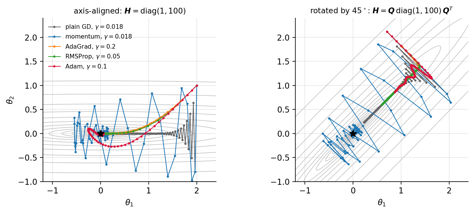
Figure 4.8: The first hundred steps of five optimisers on the quadratic bowl with Hessian eigenvalues \(1\) and \(100\), from the same starting point. Left: the Hessian is diagonal, and the adaptive methods, which rescale each coordinate by its own gradient history, move diagonally towards the minimum while plain gradient descent zigzags down the steep direction and crawls along the flat one. Right: the same bowl rotated by \(45^\circ\), with the same eigenvalues and condition number. Gradient descent and momentum are unaffected; the adaptive methods, whose diagonal rescaling cannot see the off-diagonal curvature, lose most of their advantage.
Scale invariance. A second consequence of Eq. (4.57) explains why the adaptive methods are so much less sensitive to preprocessing than gradient descent. Multiply feature \(j\), one column of the design matrix, by a constant \(c\): \(\bm{X}'=\bm{X}\bm{S}\) with \(\bm{S}=\mathrm{diag}(1,\dots,c,\dots,1)\). The least-squares cost (4.12) in the new parameters is
so the same predictions are obtained with \(\theta'_j=\theta_j/c\) and the optimum moves to \(\theta'^{*}_j=\theta^{*}_j/c\). By the chain rule, or directly from Eq. (4.13),
so that \(g'_j=c\,g_j\) while \(g'_k=g_k\) for \(k\neq j\), comparing the two problems at corresponding points \(\bm{\theta}=\bm{S}\bm{\theta}'\), and the Hessian (4.14) becomes \(\bm{H}'=\bm{S}\bm{H}\bm{S}\), with \(H'_{jj}=c^{2}H_{jj}\) and \(H'_{jk}=c\,H_{jk}\) for \(k\neq j\). For plain gradient descent the step in coordinate \(j\) is \(\Delta\theta'_j=-\gamma c\,g_j\): it grows by \(c\) while the distance to the optimum shrinks by \(c\), a mismatch of \(c^{2}\), and this is what shifts the stability bound (4.20) through \(\lambda_{\max}(\bm{H}')\), which for large \(c\) grows like \(c^{2}H_{jj}\). A learning rate that was optimal before the rescaling diverges after it. For the adaptive methods every accumulator is built from the gradient and its square, so \(r'_j=c^{2}r_j\), \(v'_j=c^{2}v_j\) and \(m'_j=c\,m_j\), and the ratios in the updates are unchanged,
The step \(\Delta\theta'_j=\Delta\theta_j\) does not depend on \(c\) at all, as long as \(g_j^{2}\gg\epsilon\), and neither does the stability of the method: the iterate takes the same steps in the rescaled units whatever the units of the data.
Why one standardises nonetheless. The invariance just derived does not make the standardisation of Chapter 3 superfluous for the adaptive methods, for three reasons. First, it is an invariance to the scaling of individual features, not to their correlation: the off-diagonal entries \(H'_{jk}=cH_{jk}\) are untouched by a diagonal \(\bm{D}_t\), which is exactly the structure the rotated bowl of Figure 4.8 showed to be out of reach. Centring the columns removes the largest single source of that correlation, the one with the intercept, and leaves \(\bm{H}\) as diagonal as the features allow. Second, the learning rate of an adaptive method is a length in the units of each parameter (Section Adam makes this precise), and a single \(\gamma\) suits every coordinate only if the parameters are of comparable size. Scaling a column by \(c\) leaves the step unchanged but makes the distance \(\theta^{*}_j/c\) it has to cover \(c\) times shorter; with \(c=100\) a coordinate whose optimum is \(0.06\) is walked at steps of \(\gamma=0.1\), straight past it. Standardised columns give parameters of the same order and let one \(\gamma\) serve all of them. Third, neither \(\epsilon\) nor a penalty is invariant. A feature scaled down until \(g_j^{2}\lesssim\epsilon\) has its denominator dominated by \(\epsilon\), and the update degenerates to \(-\gamma g_j/\sqrt{\epsilon}\), plain gradient descent with an enormous learning rate; and the Ridge cost (4.16) penalises \(\theta'^{2}_j=\theta_j^{2}/c^{2}\) instead of \(\theta_j^{2}\), so the penalty, and with it the minimiser, changes with the units – the reason Chapter 3 standardises before regularising.
4.9. AdaGrad#
AdaGrad maintains a running sum of squared gradients for each coordinate. Let \(\bm{g}_t=\nabla C_{i_t}(\bm{\theta}_t)\) be the gradient at step \(t\), possibly from a minibatch, and initialise \(\bm{r}_0=\bm{0}\). At each iteration accumulate
where \(\circ\) is the Hadamard product of Section Vectors, so that \(r_{t,j}=r_{t-1,j}+g_{t,j}^{2}\) for every coordinate \(j\). We may regard \(\bm{H}_t=\mathrm{diag}(\bm{r}_t)\) as a diagonal matrix of accumulated squared gradients, with \(\bm{H}_0=\bm{0}\).
The update scales the gradient by the inverse square root of this matrix,
where \(\bm{H}_t^{-1/2}\) is diagonal with entries \(r_{t,j}^{-1/2}\). In coordinates each parameter has its own step size,
and in practice a small constant \(\epsilon\) is added to the denominator for numerical stability,
The effective learning rate for parameter \(j\) at time \(t\) is \(\alpha_{t,j}=\gamma/\sqrt{\epsilon+r_{t,j}}\), which decreases as \(r_{t,j}\) grows.
Note the resemblance between Eq. (4.59) and Newton’s step (4.8): both premultiply the gradient by an inverse matrix built from curvature information. AdaGrad differs in using \(\bm{H}^{-1/2}\) rather than \(\bm{H}^{-1}\), in restricting \(\bm{H}\) to be diagonal, and in estimating it from gradient magnitudes rather than second derivatives.
Properties. AdaGrad tunes the step size for each parameter automatically. Parameters with large or volatile gradients receive smaller steps; those with small or infrequent gradients receive relatively larger ones. No manual schedule is needed: because \(\bm{r}_t\) never decreases, the step sizes \(\gamma/\sqrt{r_{t,j}}\) are non-increasing, which has an effect similar to a decaying learning rate but individualised per coordinate.
The benefit for sparse data is worth spelling out, since it is the setting for which AdaGrad was designed. Consider a rare feature – a word appearing in one document in a thousand. Its gradient is zero on almost every minibatch, so \(r_{t,j}\) grows very slowly, so its learning rate stays high. When the feature finally does appear, the parameter takes a large, useful step instead of the negligible one a global schedule would have permitted by then. Frequently active features, conversely, accumulate large \(r_{t,j}\) and their learning rates fall automatically.
In convex optimisation AdaGrad achieves a convergence rate comparable to the best fixed learning rate tuned in hindsight for the problem, which is a strong guarantee and effectively removes the need to tune \(\gamma\) by hand.
The built-in schedule. The form of the decay is easy to read off. Along a direction where the gradient keeps a roughly constant magnitude \(|g|\) – a flat direction far from the minimum – the accumulator is \(r_{t}\approx t\,g^{2}\) and the effective learning rate is
a \(1/\sqrt{t}\) schedule of exactly the kind that Section Learning rate schedules and stopping introduces by hand, but scaled by the size of the gradient in that coordinate, so that every direction moves by about \(\gamma/\sqrt{t}\) regardless of how steep it is. At the very first step \(r_1=g_1^{2}\) and the update is \(\gamma\,\mathrm{sign}(g_1)\) in every coordinate: the method starts by moving each parameter by the same distance \(\gamma\), whatever the gradient. This is the sense in which \(\gamma\) is a length for the adaptive methods rather than a multiplier of the gradient, a point that Section Implementations returns to. The cumulative displacement along the constant-gradient direction is \(\sum_t\gamma/\sqrt{t}\sim2\gamma\sqrt{t}\), which grows without bound but ever more slowly: AdaGrad can reach any minimum in principle, and takes increasingly long to do so in practice.
The limitation. Because \(\bm{r}_t\) accumulates without bound, the learning rates decay monotonically and can become vanishingly small long before the minimum is reached. On a convex problem this is tolerable, since the accumulated gradients genuinely reflect the geometry. In deep learning, where training runs for many epochs and the landscape changes character as the iterate moves, it is fatal: AdaGrad simply stops making progress. The sum has an infinite memory, and remembers gradients from a region of parameter space the iterate left long ago. RMSProp and Adam repair exactly this.
4.10. RMSProp#
RMSProp replaces the cumulative sum (4.58) by an exponentially decaying average,
with the square taken element-wise and \(\rho\) typically \(0.9\) or \(0.99\). The update is
with the division element-wise. The method was proposed by Geoffrey Hinton in lecture notes in 2012 and never formally published, which has not prevented it from becoming standard.
Why the change matters. Expanding Eq. (4.63) shows what has happened. Write \(\bm{g}_t=\nabla C(\bm{\theta}_t)\) for the gradient at step \(t=1,2,\dots\), start from \(\bm{v}_0=\bm{0}\) and substitute the recursion into itself,
The pattern is proved by induction: if \(\bm{v}_{t-1}=(1-\rho)\sum_{j=1}^{t-1}\rho^{\,t-1-j}\bm{g}_j^{2}\), then \(\bm{v}_t=\rho\,\bm{v}_{t-1}+(1-\rho)\bm{g}_t^{2} =(1-\rho)\sum_{j=1}^{t-1}\rho^{\,t-j}\bm{g}_j^{2}+(1-\rho)\rho^{0}\bm{g}_t^{2}\), that is,
Gradient \(\bm{g}_j\) therefore enters \(\bm{v}_t\) with the weight \(w_{t,j}=(1-\rho)\rho^{\,t-j}\), and the weights form a finite geometric series,
So \(\bm{v}_t\) is a weighted mean of the past squared gradients rather than an unbounded sum; the missing mass \(\rho^{t}\) is the weight still carried by the zero initial value \(\bm{v}_0\), a point Section Adam returns to. The mean is also a short one. A gradient that entered at step \(j\) with weight \(1-\rho\) has, \(k=t-j\) steps later, the weight \((1-\rho)\rho^{k}\), a fraction \(\rho^{k}\) of its initial weight, which has fallen below \(1/e\) once
using \(-\ln\rho=(1-\rho)+\tfrac12(1-\rho)^{2}+\dots\) for \(\rho\) close to one. For \(\rho=0.9\) this gives \(-1/\ln\rho=9.5\), so the tenth step is the first at which the weight has dropped below \(1/e\) (\(0.9^{9}=0.387\), \(0.9^{10}=0.349\)); for \(\rho=0.99\) it gives \(99.5\) and the hundredth step (\(0.99^{100}=0.366\)). Gradients older than roughly \(1/(1-\rho)\) steps – ten steps for \(\rho=0.9\), a hundred for \(\rho=0.99\) – are effectively forgotten, whereas in AdaGrad’s sum (4.58) every weight is one and the weights add up to \(t\). Two consequences follow. The quantity \(\bm{v}_t\) is now an estimate of the recent mean square gradient, so it tracks the local curvature as the iterate moves through a changing landscape. And because it does not grow without bound, the effective learning rate does not decay to zero: AdaGrad’s infinite memory problem is gone.
RMSProp is thus the same idea as AdaGrad with a finite memory, and the resemblance to the momentum update (4.28) is not accidental. Both are exponential moving averages; momentum averages the gradient, RMSProp averages its square. It is natural to ask what happens if one does both.
The price of forgetting. Finite memory removes AdaGrad’s decay, and with it AdaGrad’s ability to settle. Consider the one-dimensional quadratic \(C=\frac12\lambda\theta^{2}\) with a constant learning rate. Once the iterate is close to the minimum the gradient \(g_t=\lambda\theta_t\) is small and \(v_t\), an average of recent \(g^{2}\), is small with it: for a slowly varying iterate \(v_t\approx g_t^{2}\), and the update (4.64) becomes
a step of fixed length \(\gamma\) that cannot shrink. Convergence would require \(|\theta_{t+1}|<|\theta_t|\) for all large \(t\), that is \(\gamma\lambda/\sqrt{v_t+\epsilon}<2\); but as \(\theta_t\to0\) the denominator tends to \(\sqrt{\epsilon}\), and the condition becomes \(\gamma\lambda<2\sqrt{\epsilon}\), which with \(\epsilon=10^{-8}\) means \(\gamma\lambda<2\times10^{-4}\) – a learning rate too small to be useful. For any practical \(\gamma\) the iterate therefore ends in a limit cycle of amplitude of order \(\gamma\) around the minimum, regardless of \(\lambda\) and of \(\rho\), and the excess cost floors at a value of order \(\lambda\gamma^{2}\). On the convex polynomial fits of Section Gradient descent for linear regression this is exactly what one observes: RMSProp at a constant \(\gamma\) reaches an excess cost of \(10^{-4}\) at best and never \(10^{-6}\), at every \(\gamma\) between \(10^{-3}\) and \(1\), while AdaGrad, whose built-in \(1/\sqrt{t}\) decay of Eq. (4.62) is precisely what has been discarded, converges to rounding. RMSProp needs a decaying \(\gamma\) of the kind of Section Learning rate schedules and stopping to converge at all; in the non-convex, noisy setting of deep learning, where nobody expects to sit at a minimum, this is a price cheerfully paid for not stalling.
4.11. Adam#
Adam – adaptive moment estimation – was introduced by Kingma and Ba in 2014 [kingma2014] and does exactly that. It keeps running averages of both the first and the second moment of the gradient and uses them to adapt the learning rate for each parameter. It is efficient for large problems involving many data and many parameters, and it is the default optimiser in most deep learning frameworks.
Why combine momentum and RMSProp?. The two mechanisms address different defects and do not overlap. Momentum gives fast convergence by smoothing the gradient, accelerating along the consistent long-term direction as in Eq. (4.32) and damping oscillations across narrow valleys. RMSProp gives per-dimension scaling for stability, handling features of different scales and sparse gradients. Using both means the direction of the step is chosen by an averaged gradient while its length in each coordinate is chosen by the recent curvature estimate.
The two moments. Adam maintains, at each step \(t\),
with typical values \(\beta_1=0.9\) and \(\beta_2=0.999\), and \(\bm{m}_0=\bm{v}_0=\bm{0}\).
Bias correction. Those initialisations cause a problem which is worth deriving, because it explains a step that otherwise looks arbitrary. Equation (4.68) has the form of Eq. (4.63) with \(\rho\to\beta_2\), so the unrolled form (4.65) applies at once,
the second line being the same unrolling of Eq. (4.67). Suppose now that the gradient is stationary, with a true second moment \(\mathbb{E}[g_j^{2}]=\mathbb{E}[g^{2}]\) and a true mean \(\mathbb{E}[g_j]=\mathbb{E}[g]\) that do not depend on \(j\) (the coordinate index is suppressed). The expectation is linear, so it passes through the sum and leaves a finite geometric series,
and identically \(\mathbb{E}[m_t]=\mathbb{E}[g]\,(1-\beta_1^{\,t})\). Each raw moment is therefore too small by exactly the factor \(1-\beta_i^{t}\), which is the weight the exponential average still assigns to the zero initial value. The bias is severe at the start: with \(\beta_2=0.999\) the factor is \(10^{-3}\) at \(t=1\), so the raw \(v_1\) underestimates the true second moment by three orders of magnitude, and the step \(\gamma/\sqrt{v}\) would be enormous.
The factors \(1-\beta_1^{t}\) and \(1-\beta_2^{t}\) are deterministic: they depend on \(t\) and on the two constants, not on the data. Dividing by a constant commutes with the expectation, so
satisfy \(\mathbb{E}[\hat m_t]=\mathbb{E}[g]\) and \(\mathbb{E}[\hat v_t]=\mathbb{E}[g^{2}]\) for every \(t\ge1\), not only asymptotically: the correction removes the bias exactly, and it does so by rescaling rather than by averaging, so it adds no noise. For small \(t\) the correction is large, compensating for the initial zero; as \(t\) grows, \(1-\beta_i^{t}\to1\) and the corrected moments converge to the raw ones. The following values for the default constants show how different the two time scales are:
correction factor \(1/(1-\beta_i^{t})\) |
\(t=1\) |
\(t=10\) |
\(t=1000\) |
|---|---|---|---|
\(\beta_1=0.9\) |
\(10\) |
\(1.54\) |
\(1.00\) |
\(\beta_2=0.999\) |
\(1000\) |
\(100\) |
\(1.58\) |
The first moment is essentially unbiased after a few tens of steps, the second needs of the order of \(1/(1-\beta_2)=1000\) steps – the memory of Section RMSProp with \(\rho\to\beta_2\). Stationarity is the assumption that makes the correction exact; in a real run the gradient changes as the iterate moves, and a residual bias remains, small because the weights on old gradients are small. Bias correction is what makes Adam stable in its first iterations, and it is the one ingredient AdaGrad and RMSProp lack.
The update. Finally,
with \(\epsilon\) a small constant, typically \(10^{-8}\), preventing division by zero. Step by step: compute the gradient; update the two moving averages (4.67) and (4.68); bias-correct with Eq. (4.70); form the step \(\Delta\bm{\theta}_t=\hat{\bm{m}}_t/(\sqrt{\hat{\bm{v}}_t}+\epsilon)\); and update the parameters.
The size of an Adam step. Two properties of the update (4.71) follow from the algebra and explain much of the method’s behaviour in practice. First, at \(t=1\) the raw moments are \(\bm{m}_1=(1-\beta_1)\bm{g}_1\) and \(\bm{v}_1=(1-\beta_2)\bm{g}_1^{2}\), and the correction (4.70) divides by exactly these factors, so \(\hat{\bm{m}}_1=\bm{g}_1\) and \(\hat{\bm{v}}_1=\bm{g}_1^{2}\). The first step is then
a move of length \(\alpha\) in every coordinate, whatever the gradient – a gradient of \(10^{-3}\) and one of \(10^{3}\) produce the same first step, as for AdaGrad in Eq. (4.62). Without the correction the raw moments would enter the update directly,
with the default constants: the raw first moment is too small by a factor \(10\), the raw second moment by \(10^{3}\), and the ratio inherits \(\sqrt{10^{3}}/10=3.16\). RMSProp, which has no correction, starts with \(v_1=(1-\rho)g_1^{2}\) and Eq. (4.64) gives
a step of length \(10\gamma\) for \(\rho=0.99\) and \(3.2\gamma\) for \(\rho=0.9\), which only settles to \(\gamma\,\mathrm{sign}(g)\) after the \(1/(1-\rho)\) steps it takes the weights of Eq. (4.65) to sum to about one: one more reason for the correction. Second, at every step the magnitude of the update is bounded: since \(\hat{\bm{m}}_t\) is a weighted average of the gradients \(\bm{g}_1,\dots,\bm{g}_t\) and \(\hat{\bm{v}}_t\) a weighted average of their squares, the ratio \(|\hat m_{t,j}|/\sqrt{\hat v_{t,j}}\) is at most \((1-\beta_1)/\sqrt{1-\beta_2}\) in the worst case and at most one in the common case where the two sets of weights are comparable, so
The learning rate of Adam is a trust region: the largest distance any parameter moves in one iteration, in the units of that parameter. This is why the defaults transfer between problems as gradient descent’s \(\gamma\) never does, why Adam cannot diverge in the sense of Eq. (4.20) however \(\alpha\) is chosen (on the polynomial fit of Section Gradient descent for linear regression it converges for every \(\alpha\) between \(10^{-3}\) and \(1\), with the best value in the middle), and why its default \(\alpha=10^{-3}\) is a hundred times smaller than a typical gradient descent learning rate.
The first moment is also what lets Adam settle where RMSProp cannot. Near a minimum the gradient alternates in sign from step to step, so its average \(\hat{\bm{m}}_t\) is much smaller than its typical magnitude \(\sqrt{\hat{\bm{v}}_t}\), and the ratio in Eq. (4.71) goes to zero even at a constant \(\alpha\); the fixed-length step of Eq. (4.66) has been averaged away. On the convex problems of this chapter Adam therefore converges to rounding while RMSProp rattles. It should be added that the convergence proof in the original paper contains an error, and that Reddi, Kale and Kumar [reddi2018] constructed simple convex problems on which Adam does not converge, because the effective learning rate \(\alpha/\sqrt{\hat{\bm{v}}_t}\) can increase when a large gradient is forgotten; their repair, AMSGrad, keeps the running maximum of \(\hat{\bm{v}}_t\) instead. In practice the failure is rare and Adam as stated remains the default.
Adam against its predecessors. AdaGrad uses per-coordinate scaling like Adam but has no momentum, and slows down excessively because its accumulation never forgets. RMSProp uses a moving average of squared gradients, so it does not slow down, but includes neither momentum nor bias correction, and by Eq. (4.66) cannot settle at a constant learning rate. Adam is, in effect, RMSProp plus momentum plus bias correction: the first moment provides acceleration, smoother convergence and the ability to settle, the second moderates the step size per dimension, and the correction ensures the estimates are sound from the first iteration.
Why these methods work: the summary argument
It is worth collecting the thread that runs through Sections The learning rate and the condition number to Adam, because each method is a response to the same diagnosis.
The trouble with gradient descent is the mismatch between one global step size and a cost function whose curvature varies by direction; the iteration count scales with \(\kappa=\lambda_{\max}/\lambda_{\min}\) by Eq. (4.26). Newton’s method removes the mismatch entirely by premultiplying with \(\bm{H}^{-1}\), but costs \(\bigO(p^{3})\).
Momentum attacks the symptom: it cancels the oscillation along steep directions and accumulates progress along flat ones, improving the rate from \(\kappa\) to \(\sqrt{\kappa}\) at no extra cost. It does not, however, use different step sizes in different coordinates.
The adaptive methods attack the cause, by constructing a cheap diagonal approximation to the curvature from the second moment of the gradient. Where gradients are persistently large the curvature is presumed large and the step is shortened; where they are small the step is lengthened. Dividing by \(\sqrt{v_j}\) is an \(\bigO(p)\) stand-in for the \(\bigO(p^{3})\) operation of applying \(\bm{H}^{-1/2}\).
Two observations follow. The first is that these methods are approximately invariant to the scaling of individual features, since multiplying a feature by \(c\) multiplies its gradient by \(c\) and its accumulated second moment by \(c^{2}\), leaving the ratio unchanged. That is why they are so much less sensitive to preprocessing than plain gradient descent – although, as Section Practical tips notes, standardising the inputs remains good practice. The second is that a diagonal approximation can only capture curvature aligned with the coordinate axes. A cost function whose narrow valley runs diagonally in parameter space has a Hessian with large off-diagonal entries, and no diagonal rescaling will fix it; this is the residual gap between Adam and true second-order methods, and it is why decorrelating the inputs helps even when the scales already match.
4.12. Implementations#
The three algorithms are described in detail in Goodfellow, Bengio and Courville [goodfellow2016], chapter 8. We give compact implementations here, all applied to the same least-squares problem of Section Gradient descent for linear regression so that they may be compared directly.
import numpy as np

def make_batches(n, batch_size, rng):
    """Shuffle the indices and split them into minibatches."""
    idx = rng.permutation(n)
    return [idx[i:i + batch_size] for i in range(0, n, batch_size)]


def sgd_adaptive(X, y, method="adam", n_epochs=100, batch_size=10,
                 gamma=0.01, beta=0.9, rho=0.99,
                 beta1=0.9, beta2=0.999, eps=1e-8, rng=None):
    """Stochastic gradient descent with the optimisers of this chapter.

    method is one of "plain", "momentum", "adagrad", "rmsprop", "adam".
    """
    rng = np.random.default_rng() if rng is None else rng
    n, p = X.shape
    theta = rng.normal(size=(p, 1))

    change = np.zeros((p, 1))          # momentum velocity, Eq. (4.momentum)
    r = np.zeros((p, 1))               # accumulated second moment
    m = np.zeros((p, 1))               # first moment, Eq. (4.adamfirst)
    t = 0

    for epoch in range(n_epochs):
        for batch in make_batches(n, batch_size, rng):
            t += 1
            Xb, yb = X[batch], y[batch]
            g = (2.0 / len(batch)) * Xb.T @ (Xb @ theta - yb)

            if method == "plain":
                update = gamma * g
            elif method == "momentum":
                change = gamma * g + beta * change
                update = change
            elif method == "adagrad":
                r += g * g                                   # Eq. (4.adagradaccum)
                update = gamma * g / (np.sqrt(r) + eps)        # Eq. (4.adagrad)
            elif method == "rmsprop":
                r = rho * r + (1 - rho) * g * g              # Eq. (4.rmspropaccum)
                update = gamma * g / (np.sqrt(r) + eps)        # Eq. (4.rmsprop)
            elif method == "adam":
                m = beta1 * m + (1 - beta1) * g              # Eq. (4.adamfirst)
                r = beta2 * r + (1 - beta2) * g * g          # Eq. (4.adamsecond)
                m_hat = m / (1 - beta1**t)                   # Eq. (4.adambias)
                r_hat = r / (1 - beta2**t)
                update = gamma * m_hat / (np.sqrt(r_hat) + eps)
            else:
                raise ValueError(f"unknown method {method}")

            theta -= update

    return theta
The same five updates can be written as a single step function that
knows nothing about data, epochs or minibatches: it receives a gradient and
returns the new parameters, keeping its running quantities in a dictionary.
The data loop of the previous listing, or the full-gradient loop of
Section Gradient descent for linear regression, then calls it once per gradient. This is the
structure we recommend for the projects, because it separates the three
things that can go wrong – the cost, its gradient, and the optimiser – and
lets an analytical gradient and jax.grad of Section Automatic differentiation
be exchanged without touching the optimiser.
import numpy as np

def optimiser_step(method, theta, g, state, t, gamma, beta=0.9, rho=0.99,
                   beta1=0.9, beta2=0.999, eps=1e-8):
    """One update of theta from the gradient g at step t = 1, 2, ...; state carries the running quantities."""
    if method == "plain":                                                       # Eq. (4.gd)
        return theta - gamma * g, state
    if method == "momentum":                                                    # Eq. (4.momentum)
        state["v"] = v = beta * state.get("v", 0.0) + gamma * g
        return theta - v, state
    if method == "adagrad":                                                     # Eqs. (4.adagradaccum), (4.adagrad)
        state["r"] = r = state.get("r", 0.0) + g * g
        return theta - gamma * g / (np.sqrt(r) + eps), state
    if method == "rmsprop":                                                     # Eqs. (4.rmspropaccum), (4.rmsprop)
        state["r"] = r = rho * state.get("r", 0.0) + (1.0 - rho) * g * g
        return theta - gamma * g / (np.sqrt(r) + eps), state
    if method == "adam":                                                        # Eqs. (4.adamfirst)-(4.adam)
        state["m"] = m = beta1 * state.get("m", 0.0) + (1.0 - beta1) * g
        state["r"] = r = beta2 * state.get("r", 0.0) + (1.0 - beta2) * g * g
        m_hat, r_hat = m / (1.0 - beta1**t), r / (1.0 - beta2**t)
        return theta - gamma * m_hat / (np.sqrt(r_hat) + eps), state
    raise ValueError(f"unknown method {method}")

def optimise(grad, theta0, method, gamma, num_iters=1000, tol=1e-8, **kw):
    """Full-gradient loop around optimiser_step; returns every iterate."""
    theta, state = np.array(theta0, dtype=float), {}
    history = [theta.copy()]
    for t in range(1, num_iters + 1):
        g = grad(theta)
        theta, state = optimiser_step(method, theta, g, state, t, gamma, **kw)
        history.append(theta.copy())
        if np.linalg.norm(g) < tol:
            break
    return np.array(history)
Running all five on the data of Section Gradient descent for linear regression for a hundred epochs with batches of ten, for three values of the learning rate, gives the final cost values of Table 4.4. The analytical solution of Eq. (3.8) is \(\hat{\bm{\theta}}=(4.030,2.806)\) with cost \(1.14947\), which is the floor.
Method |
\(\gamma=0.01\) |
\(\gamma=0.1\) |
\(\gamma=0.5\) |
|---|---|---|---|
Plain SGD |
\(1.1499\) |
\(1.1532\) |
\(1.2274\) |
Momentum |
\(1.1553\) |
\(1.5674\) |
\(1.3490\) |
AdaGrad |
\(28.049\) |
\(1.2776\) |
\(\mathbf{1.1497}\) |
RMSProp |
\(1.1516\) |
\(1.1512\) |
\(1.1904\) |
Adam |
\(1.2185\) |
\(1.1514\) |
\(1.1565\) |
Table 4.4: Final value of the cost function (4.12) after \(100\) epochs of stochastic gradient descent on the data of Section Gradient descent for linear regression, for each optimiser and three learning rates. The analytical minimum is \(1.14947\). Note that no row is best at the same \(\gamma\) as any other.
The table repays study, and not because it flatters the adaptive methods.
The first observation is that on this problem the sophisticated methods are not better. With \(\gamma=0.01\) plain SGD reaches \(1.1499\), within \(0.04\%\) of the optimum, while Adam manages only \(1.2185\) and AdaGrad is catastrophic at \(28.05\) – it has not arrived anywhere near the minimum. This is exactly what Section AdaGrad predicted: the accumulated \(\bm{r}_t\) drives the effective step \(\gamma/\sqrt{r_t}\) towards zero, and with \(\gamma\) already small the iterate stalls long before reaching the solution. Nothing is wrong with the implementation; the method is behaving as designed, and the design is wrong for this problem.
The second observation explains the first. Look along the rows rather than down the columns. AdaGrad is worst at \(\gamma=0.01\) and best of all five at \(\gamma=0.5\), where it essentially attains the analytical minimum. Plain SGD and momentum move the other way, degrading as \(\gamma\) grows. The reason is that these methods do not use \(\gamma\) to mean the same thing. Plain gradient descent multiplies \(\gamma\) by the raw gradient, so the stability bound (4.20) applies directly. The adaptive methods divide by \(\sqrt{v_j}\) first, which renormalises the gradient to something of order unity, so their \(\gamma\) sets a step length in parameter space rather than a multiple of the gradient. A learning rate is not comparable across optimisers, and a comparison at a single fixed \(\gamma\) – which is what one sees most often – says more about which method happens to suit that number than about the methods.
The third observation is the one to carry forward. This problem has \(p=2\), is convex, and has a Hessian with eigenvalues \(0.311\) and \(3.728\), hence \(\kappa=11.97\) by Eq. (4.26). That is a benign landscape, and there is simply nothing for the adaptive machinery to repair; the overhead of estimating curvature buys nothing because the curvature is already uniform. The adaptive methods earn their place when \(\kappa\) is large, when \(p\) is large, when the gradients are sparse, and when the cost is non-convex – which is to say in the neural networks of the following chapters, and not here. Demonstrating a method on a problem it was not designed for is a good way to understand what it actually does.
Figure 4.9 plots the same comparison as a function of the epoch rather than as a final number, and it makes the second lesson of the table unmistakable. At \(\gamma=0.01\) the adaptive methods are slower than plain stochastic gradient descent and AdaGrad has effectively stopped; at \(\gamma=0.5\) the ordering is reversed and AdaGrad is the best of the five. Nothing about the methods has changed between the panels. Only the number \(\gamma\) has, and it means something different to each of them.
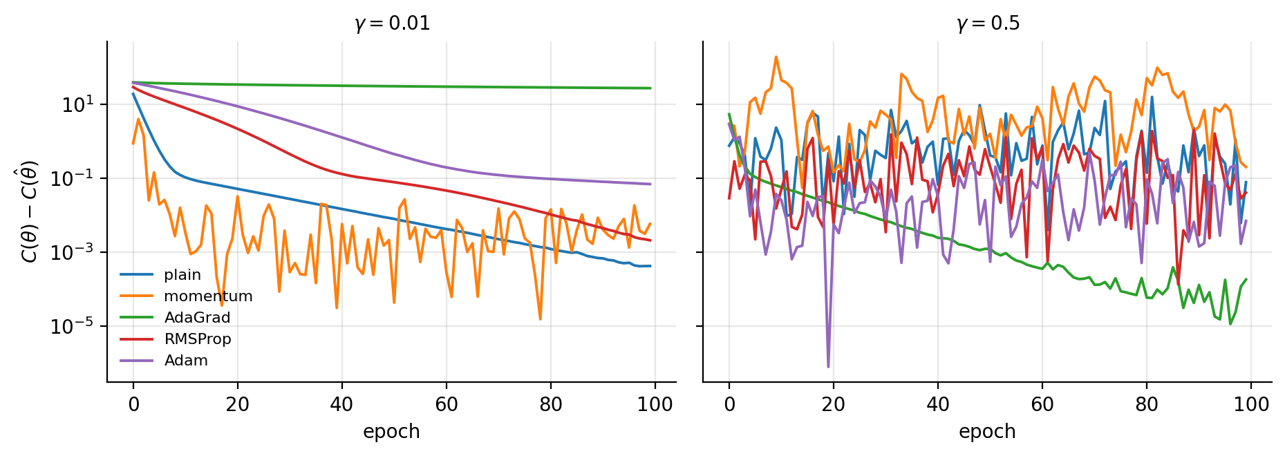
Figure 4.9: Excess cost against epoch for the five optimisers of Section Implementations at two learning rates. The vertical axis is \(C(\bm{\theta})\) minus its value at the analytical minimum. The ranking of the methods reverses between the panels.
Machine learning connection
The default hyperparameters \(\beta_1=0.9\), \(\beta_2=0.999\), \(\epsilon=10^{-8}\) and \(\alpha=10^{-3}\) from the original paper are used almost universally and are usually a reasonable starting point, which is a large part of Adam’s popularity. It should be said, however, that adaptive methods do not always generalise as well as plain SGD. Several studies have found that models trained with Adam, RMSProp or AdaGrad reach a worse test error than the same models trained with well-tuned SGD with momentum, particularly in the overparameterised regime where the number of parameters exceeds the number of data points. Why this should be so is not settled. The practical advice is that Adam is an excellent default for getting a model training at all, and that a carefully tuned SGD with momentum is worth trying before the final result is reported.
4.13. None of these can compete with Newton’s method#
It is a useful corrective, having built up this machinery, to see how it fares against Eq. (4.8) on a problem where the Hessian is affordable. For the least-squares cost of Section Gradient descent for linear regression a single Newton step lands on the exact minimum, by Eq. (4.9), while the methods above need hundreds or thousands of iterations to get five decimal places.
import numpy as np

# One Newton step solves the least-squares problem exactly
H = (2.0 / n) * X.T @ X
theta = rng.normal(size=(2, 1))
gradient = (2.0 / n) * X.T @ (X @ theta - y)
theta -= np.linalg.solve(H, gradient)
print("after one Newton step:", theta.ravel())
print("analytical solution:  ", (np.linalg.pinv(X.T @ X) @ X.T @ y).ravel())
The two agree to machine precision. The moral is not that we should use Newton’s method – for a quadratic cost we would use the closed form of Chapter 3, and for a large model we could not afford the Hessian at all – but that the gradient methods of this chapter are approximations to something better, adopted because of cost. Every improvement from momentum to Adam is a step back towards Eq. (4.8), recovering a little more curvature information for a little more bookkeeping, and the quality of a method can fairly be judged by how much of the Hessian it manages to imitate for \(\bigO(p)\) work per step.
4.14. Automatic differentiation#
Every method in this chapter needs a gradient. For linear regression we
computed it by hand in Eq. (4.13); for a neural network with
a dozen layers, doing so by hand is possible but error-prone, and for a model
under active development it is impractical. Automatic differentiation
(AD), also called algorithmic differentiation, solves the problem completely,
and this section explains how. We first say precisely what AD is not, then
derive its two modes from the chain rule, prove the one result about cost that
makes deep learning feasible, and finally show how the same ideas are used
from Python through the JAX library.
AD exploits the fact that every computer program, however complicated, executes a sequence of elementary arithmetic operations and elementary functions – addition, multiplication, \(\exp\), \(\log\), \(\sin\) – each of whose derivatives is known. Applying the chain rule of Eq. (1.51) repeatedly to that sequence yields derivatives of arbitrary order, accurate to working precision, at a cost only a small constant factor above that of the original program. Both halves of that sentence – the accuracy and the cost – are theorems, and we shall prove them.
4.14.1. Three ways to differentiate a program#
It is important to distinguish AD from the two things it is often confused with.
Symbolic differentiation. A symbolic differentiator manipulates expressions: it takes the formula for \(f\) and returns the formula for \(f'\). This is what a computer-algebra system does and it is exact, but it requires the program to be a single closed-form expression in the first place – no loops, no branches, no intermediate variables – and it suffers from expression swell: the derivative of a product of \(m\) factors has \(m\) terms, the derivative of that has \(m^{2}\), and the size of the formula grows without any of the sharing of intermediate results that the original program enjoyed.
Numerical differentiation. A numerical differentiator replaces the derivative by a difference quotient. For a function of one variable the central difference is
and its error can be analysed exactly. Expanding both terms in Taylor series about \(x\) and subtracting, all even powers of \(h\) cancel and
the truncation error, which shrinks as \(h^{2}\). This suggests taking \(h\) as small as possible. But the two function values are computed in floating point, each with a relative error of order the unit roundoff \(\epsilon_M\approx2.2\times10^{-16}\) of Section Vector and matrix norms, so the numerator carries an absolute error of order \(\epsilon_M|f(x)|\) and the quotient an error of order \(\epsilon_M|f(x)|/h\): the rounding error, which grows as \(h\) shrinks. This is catastrophic cancellation, the subtraction of two nearly equal numbers. The total error is therefore of the form
and setting \(dE/dh=0\) gives the optimal step and the best attainable accuracy,
A central difference can never deliver more than about two thirds of the available digits, and only if \(h\) is chosen well; the one-sided difference \((f(x+h)-f(x))/h\) has truncation error \(\bigO(h)\) and does correspondingly worse, \(E\sim\epsilon_M^{1/2}\approx10^{-8}\). Figure 4.12 shows the curve (4.75) measured for a concrete function. And the cost is the second objection: for a function of \(p\) variables the gradient needs \(2p\) evaluations, or \(p+1\) for one-sided differences, and for \(p=10^{7}\) that is a week of computing to obtain one, mediocre, gradient.
Automatic differentiation. AD has neither defect. It computes the numerical value of the derivative at a point, not a formula, so there is no expression swell; it does so by propagating exact derivative rules through the program, so there is no truncation error and no step \(h\) to choose; and, in the mode used for training, it obtains all \(p\) components of the gradient for the price of a small constant number of evaluations of \(f\). Reverse-mode AD is what backpropagation is. For \(p=10^{7}\) the difference against finite differences is between a fraction of a second and a week, and it is the reason the models of the later chapters can be trained at all.
4.14.2. Evaluation traces and the computational graph#
The object AD works on is not the formula for \(f\) but the sequence of operations a program executes to evaluate it. Consider the function
which a program evaluates as the following list of assignments, each applying one elementary operation \(\varphi_i\) to variables already computed:
This is the evaluation trace, or Wengert list, of \(f\) [wengert1964,griewank2008]: the inputs are numbered \(v_{1-n},\dots,v_0\), the intermediate results \(v_1,\dots,v_\ell\) in the order in which they are computed, and the output is the last of them. Drawn as a directed graph with an edge \(j\to i\) whenever \(v_i\) depends directly on \(v_j\), it is the computational graph of Fig. 4.10. Any program made of elementary operations has such a trace – loops unroll into repeated assignments, and a branch simply selects which assignments are executed for the given input – and that is what makes AD applicable to programs rather than to formulae. A neural network is a particularly regular trace: the matrix products, additions and activation functions of Chapter 8, one layer after another.
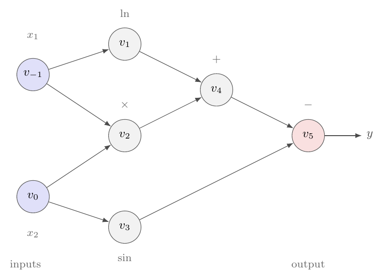
Figure 4.10: The computational graph of the evaluation trace (4.78) for \(f(x_1,x_2)=\ln x_1+x_1x_2-\sin x_2\). Each node is one elementary operation applied to its predecessors. Forward-mode AD sweeps this graph from left to right, carrying a derivative \(\dot v_i\) with every value; reverse-mode AD first evaluates the values from left to right and then sweeps back from right to left, carrying an adjoint \(\bar v_i=\partial y/\partial v_i\) with every node.
For each node the derivative of the elementary operation with respect to each of its arguments – its local or partial derivative – is known in closed form:
Everything AD does is to combine these local derivatives by the chain rule. The only question is in which order, and there are two natural answers.
4.14.3. Forward mode: tangents and dual numbers#
Fix a direction \(\dot{\bm{x}}\in\mathbb{R}^{n}\) in the input space and define for every node its tangent, the directional derivative
Since \(v_i=\varphi_i(v_j:j\prec i)\) depends only on its predecessors, the chain rule gives the forward recursion
started from \(\dot v_{1-n},\dots,\dot v_0\) set equal to the chosen direction \(\dot x_1,\dots,\dot x_n\). The recursion runs in the same order as the evaluation itself, so each tangent can be computed alongside its value, and when the sweep reaches the output it holds \(\dot y=\nabla f(\bm{x})^{T}\dot{\bm{x}}\). For our example with \(\dot{\bm{x}}=(1,0)\), that is \(\partial f/\partial x_1\), the sweep at \((x_1,x_2)=(2,5)\) reads
and indeed \(\partial f/\partial x_1 = 1/x_1 + x_2 = 5.5\). To obtain \(\partial f/\partial x_2\) the whole sweep is repeated with \(\dot{\bm{x}}=(0,1)\).
Dual numbers. There is an elegant algebraic way to say the same thing. Introduce a symbol \(\varepsilon\) with \(\varepsilon^{2}=0\) (but \(\varepsilon\neq0\)) and consider dual numbers \(a+b\varepsilon\) with \(a,b\in\mathbb{R}\). They add componentwise and multiply as
because the \(\varepsilon^{2}\) term vanishes. Now let \(g\) be any function with a Taylor series and evaluate it at a dual argument. Every power of \(\varepsilon\) beyond the first is zero, so the series terminates:
The dual part is exactly the tangent (4.81) of \(g\): dual numbers carry a value and a derivative together, and the multiplication rule (4.83) is the product rule. Applying \(g\) to \(x+1\cdot\varepsilon\) and reading off the coefficient of \(\varepsilon\) therefore returns \(g'(x)\) exactly – not approximately, since nothing was truncated: the series terminates by the algebra of \(\varepsilon\), not by neglecting small terms. This is forward-mode AD in one line, and it can be implemented in a few more. The following class overloads the arithmetic operators of Python so that ordinary code, written with no thought of derivatives, computes them when handed a dual argument.
import math

class Dual:
    """A dual number a + b*eps with eps**2 = 0: a value and its derivative."""
    def __init__(self, val, dot=0.0):
        self.val, self.dot = val, dot
    def _lift(o):                       # promote plain floats to duals
        return o if isinstance(o, Dual) else Dual(o)
    def __add__(self, o):
        o = Dual._lift(o); return Dual(self.val + o.val, self.dot + o.dot)
    __radd__ = __add__
    def __sub__(self, o):
        o = Dual._lift(o); return Dual(self.val - o.val, self.dot - o.dot)
    def __mul__(self, o):               # the product rule, Eq. (4.dualmult)
        o = Dual._lift(o)
        return Dual(self.val * o.val, self.val * o.dot + self.dot * o.val)
    __rmul__ = __mul__
    def __truediv__(self, o):           # the quotient rule
        o = Dual._lift(o)
        return Dual(self.val / o.val,
                    (self.dot * o.val - self.val * o.dot) / o.val**2)
    def __pow__(self, k):
        return Dual(self.val**k, k * self.val**(k - 1) * self.dot)

# elementary functions: value and local derivative, Eq. (4.dualtaylor)
def sin(d): return Dual(math.sin(d.val), math.cos(d.val) * d.dot)
def exp(d): return Dual(math.exp(d.val), math.exp(d.val) * d.dot)
def log(d): return Dual(math.log(d.val), d.dot / d.val)

def f(x1, x2):                          # Eq. (4.adexample), ordinary code
    return log(x1) + x1 * x2 - sin(x2)

# seed the tangent of the variable we differentiate with respect to
print("df/dx1 =", f(Dual(2.0, 1.0), Dual(5.0, 0.0)).dot)   # 1/x1 + x2 = 5.5
print("df/dx2 =", f(Dual(2.0, 0.0), Dual(5.0, 1.0)).dot)   # x1 - cos(x2)
print("exact  =", 0.5 + 5.0, 2.0 - math.cos(5.0))
Jacobian–vector products and the cost of forward mode. For a vector-valued \(\bm{f}:\mathbb{R}^{n}\to\mathbb{R}^{m}\) with Jacobian \(\bm{J}\in\mathbb{R}^{m\times n}\) as in Eq. (1.16), one forward sweep with seed \(\dot{\bm{x}}\) returns
a Jacobian–vector product (JVP), without ever forming \(\bm{J}\). Seeding with the unit vector \(\bm{e}_k\) returns the \(k\)-th column of the Jacobian, so the full Jacobian costs \(n\) sweeps and the gradient of a scalar function of \(p\) parameters costs \(p\) sweeps – the same count as finite differences, only exact. Each sweep costs a small multiple of one function evaluation, since Eq. (4.81) adds to each elementary operation a bounded number of further ones. Forward mode is therefore the right tool when the number of inputs is small: the sensitivity of a whole network output to one physical parameter, or the derivatives with respect to one or two spatial coordinates that Chapter 9 needs when a network is made to satisfy a differential equation. It is the wrong tool for training, where \(p\) is enormous and the output is a single scalar.
4.14.4. Reverse mode: adjoints#
Reverse mode fixes the output instead of the input. For a scalar output \(y\) define the adjoint of every node,
the sensitivity of the final result to that intermediate value. Since \(y\) depends on \(v_j\) only through the nodes \(v_i\) that consume it, the chain rule gives the reverse recursion
started from \(\bar v_\ell=\partial y/\partial y=1\). Compare this with the forward recursion (4.81): the same local derivatives appear, but the sum now runs over the successors of a node and the recursion runs backwards through the trace, from output to inputs. When it reaches the inputs it holds \(\bar v_{1-n},\dots,\bar v_0\), which is the whole gradient \(\nabla f(\bm{x})\) – all \(n\) components from a single sweep. For our example, with the values from the forward evaluation at \((2,5)\),
which are \(\partial f/\partial x_2\) and \(\partial f/\partial x_1\), both obtained at once. The two contributions to \(\bar v_0\) are the two paths from \(v_0\) to \(y\) in Fig. 4.10: the chain rule sums over paths, and the reverse sweep organises that sum so that each edge is visited once.
Reverse mode has a price that forward mode does not: the local derivatives in Eq. (4.87) depend on the values \(v_j\) – \(\cos v_0\), \(v_{-1}\), \(1/v_{-1}\) above – and those must be available when the backward sweep needs them, in the reverse of the order in which they were produced. The forward evaluation must therefore be recorded, on what is called the tape, and the memory cost of reverse mode is proportional to the length of the trace rather than to the number of variables. This is why training a deep network is memory-bound: every activation of every layer is stored until the backward pass has consumed it.
Vector–Jacobian products. For a vector-valued function seeded with a covector \(\bar{\bm{y}}\in\mathbb{R}^{m}\) the reverse sweep returns
a vector–Jacobian product (VJP): one row of \(\bm{J}\) per sweep, and the full Jacobian in \(m\) sweeps. Equation (4.89) is precisely Eq. (1.51), a gradient propagated backwards by multiplication with a transposed Jacobian, and it is why backpropagation was described in Section The chain rule as the chain rule with the products taken in the cheapest order.
The cheap gradient principle. The result that makes all of deep learning possible is the following.
Proposition 4.2 (Cheap gradient principle)
Let \(f:\mathbb{R}^{p}\to\mathbb{R}\) be evaluated by a trace of \(\ell\) elementary operations, each of which has at most two arguments and whose local derivatives cost at most a fixed multiple of the operation itself. Then reverse-mode AD computes \(f(\bm{x})\) and the complete gradient \(\nabla f(\bm{x})\) with at most \(c\,\ell\) operations, where \(c\le4\) is a constant independent of \(p\).
Proof
The forward evaluation costs \(\ell\) operations and records the trace. In the reverse recursion (4.87) each edge \(j\to i\) of the graph contributes exactly one term \(\bar v_i\,\partial\varphi_i/\partial v_j\): one multiplication, one addition into \(\bar v_j\), and the evaluation of the local derivative, which by hypothesis costs a bounded amount and often nothing at all (for \(+\) it is \(1\), for \(\times\) it is the other argument, already on the tape). Since each node has at most two incoming edges, the number of edges is at most \(2\ell\) and the reverse sweep costs at most a fixed multiple of \(2\ell\) operations. Adding the forward evaluation gives the bound, and nowhere did \(p\) enter: it determines how many adjoints are read off at the end, not how many operations are performed.
The result is due to Baur and Strassen [baur1983] in the setting of arithmetic circuits and to Linnainmaa [linnainmaa1976] and, independently, the backpropagation literature in the setting of programs; the survey by Baydin et al. [baydin2018] traces the history. In practice the constant is nearer \(2\)–\(3\) than \(4\): a gradient costs about as much as two or three function evaluations. Set against the \(p+1\) evaluations of finite differences or the \(p\) sweeps of forward mode, this is the entire difference between what can and cannot be trained.
Machine learning connection
Backpropagation, the algorithm of Chapter 8 that trains every neural network, is Eq. (4.87) specialised to the layered trace of a network. The forward pass computes and stores the activations; the backward pass propagates the adjoint of the cost – the “error” of the older literature – from the output layer to the input, one transposed weight matrix at a time, exactly as in Eq. (4.89). Nothing in backpropagation is specific to networks: it is reverse-mode AD, and modern frameworks make no distinction.
4.14.5. Two examples worked by hand#
The example of Eq. (4.77) had two inputs, which is what makes the difference between the two modes visible. It is nevertheless worth running both sweeps on two functions of a single variable, small enough that every number can be checked against the derivative one would write down by hand, because they show the two things a first encounter with AD tends to obscure: that the sweeps only ever multiply and add numbers already on the tape, and that the reverse sweep has to sum whenever a value is used more than once.
A chain. Take first
whose trace has a single input and two intermediate values,
with local derivatives \(\partial v_1/\partial v_0=2v_0\) and \(\partial v_2/\partial v_1=\exp v_1=v_2\). The computational graph, upper panel of Fig. 4.11, is a chain: every node has one predecessor and one successor. The forward recursion (4.81) seeded with \(\dot v_0=1\) reads
and the reverse recursion (4.87) started from \(\bar v_2=1\) reads
Both are the chain rule \(df/dx=(df/dv_2)(dv_2/dv_1)(dv_1/dv_0)\); forward mode multiplies the three factors from the right, reverse mode from the left, and on a chain the two are indistinguishable in cost. Evaluating \(f\) takes two elementary operations, a square and an exponential. Either sweep adds two multiplications, and notice that \(\exp(x^{2})\) is not recomputed: it is \(v_2\), read off the tape. At \(x=1\) all three agree on \(f'(1)=2e=5.437\).
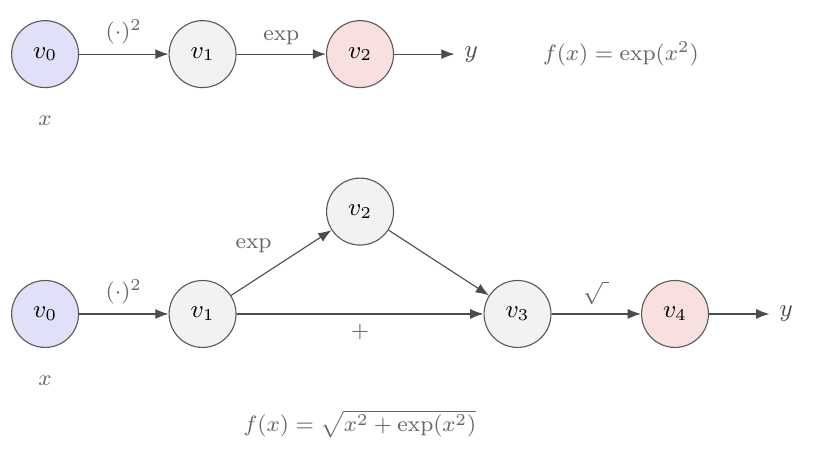
Figure 4.11: The computational graphs of the two examples of Section Two examples worked by hand. Top: \(f(x)=\exp(x^{2})\), trace (4.91), a chain in which every value is used once. Bottom: \(f(x)=\sqrt{x^{2}+\exp(x^{2})}\), trace (4.95), where \(v_1=x^{2}\) feeds both the exponential and the sum. The two paths from \(v_1\) to \(y\) are the two terms of the adjoint \(\bar v_1\) in Eq. (4.97).
A fan-out. The second function reuses an intermediate value,
with the trace
shown in the lower panel of Fig. 4.11. The node \(v_1\) now has two successors, \(v_2\) and \(v_3\), and this is where the two modes part company. The forward sweep is unaffected – each node still collects tangents from its predecessors, and \(v_3\) simply has two of them:
The reverse sweep starts from \(\bar v_4=1\) and walks back through the trace,
and the adjoint of \(v_1\) is a sum of two terms, one through each successor, exactly as Eq. (4.87) prescribes: the sensitivity of \(y\) to \(v_1\) is the sensitivity through the exponential plus the sensitivity through the direct addition. Substituting \(v_2=\exp(x^{2})\) and \(v_3=x^{2}+\exp(x^{2})\) gives
which is what the chain rule applied by hand produces. At \(x=1\) the tape holds \(v_1=1\), \(v_2=2.718\), \(v_3=3.718\) and \(v_4=1.928\), and both sweeps return \(f'(1)=3.718/1.928=1.928\). (That \(f'(1)\) equals \(f(1)\) is a coincidence of the point \(x=1\), where the numerator \(x(1+v_2)\) happens to equal \(v_3\).)
The bookkeeping is worth comparing. Evaluating \(f\) costs four elementary operations. The reverse sweep adds two for \(\bar v_3\), two for \(\bar v_1\) and two for \(\bar v_0\), six in all, and every quantity it needs – \(v_2\), \(v_4\), \(v_0\) – is already on the tape. Evaluating the closed form (4.98) on its own, without sharing anything with the evaluation of \(f\), costs about eight operations and computes \(x^{2}\) and \(\exp(x^{2})\) a second time; on a function with thousands of intermediate values the hand-derived expression grows far faster than the trace, which is the expression swell that AD avoids by never forming it. Both sweeps here are within the constant of Proposition 4.2, and the reader can check that the same holds for the example of Fig. 4.10.
The following listing runs the two examples through the Dual class
of Section Forward mode: tangents and dual numbers for the forward sweep and through JAX for
the reverse sweep (Section Automatic differentiation in Python: autograd and JAX says more about JAX), and
compares both with Eq. (4.98). The functions are
written exactly as one would write them without derivatives in mind.
import math
import jax
import jax.numpy as jnp
jax.config.update("jax_enable_x64", True)

def sqrt(d):                            # one more elementary function for Dual
    r = math.sqrt(d.val)
    return Dual(r, d.dot / (2.0 * r))

def f_chain(x):                         # Eq. (4.adchainfun)
    return exp(x**2)

def f_fanout(x):                        # Eq. (4.adfanoutfun)
    a = x**2
    return sqrt(a + exp(a))

x = 1.0
# forward mode: seed the tangent of x with 1 and read the dual part
print("chain,   forward:", f_chain(Dual(x, 1.0)).dot, " exact:", 2 * x * math.exp(x**2))
print("fan-out, forward:", f_fanout(Dual(x, 1.0)).dot)

# reverse mode: jax.grad is one reverse sweep, Eq. (4.adfanoutreverse)
def f_fanout_jax(x):
    a = x**2
    return jnp.sqrt(a + jnp.exp(a))

print("fan-out, reverse:", float(jax.grad(f_fanout_jax)(x)))
print("fan-out, closed: ", x * (1 + math.exp(x**2)) / math.sqrt(x**2 + math.exp(x**2)))
The three numbers agree to rounding, \(1.92828468553247\), differing at most in the last binary digit: nothing was approximated in either sweep.
4.14.6. Forward or reverse: the chain rule as a matrix product#
The cleanest way to see why the two modes differ in cost is to write a program as a composition of \(L\) stages, \(\bm{f}=\bm{f}_L\circ\bm{f}_{L-1}\circ\cdots\circ\bm{f}_1\), with \(\bm{f}_k:\mathbb{R}^{n_{k-1}}\to\mathbb{R}^{n_k}\), \(n_0=n\) and \(n_L=m\). The chain rule of Eq. (1.50) says that the Jacobian is a product of the stage Jacobians,
Matrix multiplication is associative, so this product may be evaluated in any order, and the orders differ enormously in cost. Forward mode multiplies from the right, \(\bm{J}\dot{\bm{x}}=\bm{J}_L(\cdots(\bm{J}_2(\bm{J}_1\dot{\bm{x}})))\), so every intermediate is a vector of length \(n_k\) and never a matrix. Reverse mode multiplies from the left, \(\bar{\bm{y}}^{T}\bm{J} =(((\bar{\bm{y}}^{T}\bm{J}_L)\bm{J}_{L-1})\cdots)\bm{J}_1\), and again every intermediate is a vector. If the stage Jacobians are dense the cost of the right-to-left product is \(\sum_k n_kn_{k-1}\) per column, hence \(n\sum_kn_kn_{k-1}\) for the whole Jacobian, while the left-to-right product costs \(m\sum_kn_kn_{k-1}\). The rule is therefore simple: use forward mode when \(n\ll m\) and reverse mode when \(m\ll n\). Training a model is the extreme case \(m=1\), \(n=p\), and reverse mode wins by a factor \(p\). When \(n\) and \(m\) are comparable, neither mode is optimal and finding the cheapest bracketing of Eq. (4.99) – the optimal Jacobian accumulation problem – is NP-hard, though good heuristics exist [griewank2008].
Second derivatives. The two modes compose, and their composition gives cheap access to curvature. The Hessian of a scalar \(f\) is the Jacobian of its gradient, and the Hessian–vector product is a directional derivative of the gradient,
The right-hand side is a forward-mode derivative, in the direction \(\bm{v}\),
of a function – the gradient – that is itself computed by reverse mode.
This forward-over-reverse construction costs a small constant times
one gradient, hence a small constant times one function evaluation, and it
never forms the \(p\times p\) Hessian. That is exactly the price at which
Section None of these can compete with Newton’s method said curvature information could not
be had; the truncated-Newton and conjugate-gradient methods of the
optimisation literature [nocedal2006] use Eq. (4.100) to run
Newton’s method (4.8) with only Hessian–vector products,
and the natural-gradient methods of Chapter 8 rely on the same
device. The full Hessian, when it is wanted, is \(p\) such products,
\(\bm{H}=\bm{H}[\bm{e}_1,\dots,\bm{e}_p]\), and this is how
jax.hessian computes it.
4.14.7. Accuracy, and points where the derivative does not exist#
We claimed that AD is accurate to working precision, and the claim can now be made precise. The recursions (4.81) and (4.87) are exact identities; the only errors are the rounding errors of the floating-point operations that implement them. Each tangent or adjoint is obtained from its predecessors by a short chain of multiplications and additions of quantities that were themselves computed to relative accuracy \(\bigO(\epsilon_M)\), so the derivative inherits the numerical stability of the function evaluation itself: if the program computes \(f\) to \(d\) correct digits it computes \(\nabla f\) to about \(d\) correct digits as well. There is no step \(h\), no cancellation of nearly equal numbers, and no term of the form \(\epsilon_M/h\). In Fig. 4.12 the AD derivative sits at the floor of the plot, at \(10^{-16}\), for the same reason that the function value does.
The one genuine limitation is that AD differentiates the program actually executed. At a point where the function is not differentiable – \(|x|\) at zero, or the ReLU activation \(\max(0,x)\) of Chapter 8 at \(x=0\) – the program takes one of the two branches and AD returns the derivative of that branch, typically \(0\) or \(1\) by convention. This is a valid subgradient and is harmless in practice, since the set of such points has measure zero and an iterate never lands on it exactly. More insidious is a program that computes a smooth function by a non-smooth route, for instance \(\sqrt{x^{2}}\) for \(|x|\) or a table lookup with interpolation, whose AD derivative is that of the route rather than of the function. Writing functions with AD in mind – using the library’s own \(\log(1+e^{x})\), \(\log\sum\exp\) and similar numerically careful primitives, whose derivative rules are hand-written – avoids both this and overflow in intermediate values.
4.14.8. Automatic differentiation in Python: autograd and JAX#
Two libraries deliver the machinery above to ordinary numpy code. The older
autograd package overloads the numpy functions with dual-number-like
objects that record a tape, exactly as the Dual class above did for
the standard library, and it remains a good way to see the mechanism at work:
import autograd.numpy as np
from autograd import grad

def f(x):
    return np.sin(2 * np.pi * x + x**2)

df = grad(f)                 # df is a Python function, the derivative of f
print(df(1.0))               # (2 pi + 2) cos(2 pi + 1) = 4.475424121402227

# It composes: the second derivative is just grad applied twice
d2f = grad(grad(f))
print(d2f(1.0))
For current work we recommend JAX [jax2018]. JAX combines the
same differentiation machinery with a compiler, XLA, so that the resulting
code can additionally be just-in-time compiled, vectorised over a batch and
run on GPUs and TPUs, and it exposes forward mode, reverse mode and their
compositions explicitly. Its four fundamental transformations are
grad, jit, vmap and the pair jvp and
vjp, and they compose freely.
Precision
JAX uses single precision by default. Every numerical
comparison in this book is made in double precision, and the first line of
every JAX program should therefore be
jax.config.update("jax_enable_x64", True). Without it the
gradient checks below would agree only to about seven digits and one would
wrongly conclude that AD is inexact.
import jax
jax.config.update("jax_enable_x64", True)   # double precision throughout
import jax.numpy as jnp
from jax import grad, jit, vmap

def f(x):
    return jnp.sin(2 * jnp.pi * x + x**2)

df = grad(f)                       # reverse-mode gradient of a scalar function
print(df(1.0))                     # 4.475424121402227, exact to all digits
print(grad(grad(f))(1.0))          # second derivative, by composing grad

xs = jnp.linspace(0.0, 1.0, 5)
print(vmap(df)(xs))                # the derivative at five points at once
fast_df = jit(df)                  # compiled on first call, then very fast
print(fast_df(1.0))
Forward and reverse mode explicitly.
The two modes of Sections Forward mode: tangents and dual numbers and Reverse mode: adjoints are
available directly. jvp takes a function, a point and a tangent
direction and returns the value and the Jacobian–vector product of
Eq. (4.85); vjp takes a function and a point and returns
the value and a function that maps a covector to the vector–Jacobian product
of Eq. (4.89). jacfwd and jacrev assemble the
full Jacobian by the two routes of Section Forward or reverse: the chain rule as a matrix product, one column or
one row per sweep, and agree to rounding.
from jax import jvp, vjp, jacfwd, jacrev

def F(x):                          # a map from R^2 to R^3
    return jnp.array([x[0] * x[1], jnp.sin(x[0]), jnp.exp(x[1])])

x0 = jnp.array([1.0, 2.0])
J = jacfwd(F)(x0)                  # 3 x 2 Jacobian, built from two forward sweeps
print(J)
print(jnp.allclose(J, jacrev(F)(x0)))       # ...and from three reverse sweeps

v = jnp.array([1.0, 0.0])          # a direction in the input space
_, Jv = jvp(F, (x0,), (v,))        # forward mode: J v, first column of J
print(Jv)

u = jnp.array([1.0, 1.0, 1.0])     # a covector in the output space
_, vjp_fn = vjp(F, x0)
print(vjp_fn(u)[0])                # reverse mode: u^T J, the column sums of J
The least-squares gradient without deriving it. Applied to our least-squares problem, the gradient we derived by hand in Eq. (4.13) need never be written down. We write the cost (4.12) as a function of \(\bm{\theta}\) and the data, differentiate with respect to its first argument, compile the result, and run the gradient descent iteration (4.15) with it.
import jax
jax.config.update("jax_enable_x64", True)
import jax.numpy as jnp
import numpy as np
from jax import grad, jit

# The data of Section 4.gdlinreg
n = 100
rng = np.random.default_rng(2024)
x = 2.0 * rng.random((n, 1))
y = 4.0 + 3.0 * x + rng.normal(size=(n, 1))
X = np.c_[np.ones((n, 1)), x]
Xj, yj = jnp.asarray(X), jnp.asarray(y)

def cost(theta, X, y):                     # Eq. (4.gdcost)
    return jnp.sum((X @ theta - y)**2) / len(y)

cost_grad = jit(grad(cost, argnums=0))     # d cost / d theta, compiled

# Check against the hand-derived gradient, Eq. (4.gdgradient)
theta = jnp.asarray(rng.normal(size=(2, 1)))
g_ad = cost_grad(theta, Xj, yj)
g_hand = (2.0 / n) * X.T @ (X @ np.asarray(theta) - y)
print("max |AD - hand| =", np.max(np.abs(np.asarray(g_ad) - g_hand)))

# Gradient descent, Eq. (4.gditeration), with the automatic gradient
gamma = 0.1
@jit
def gd_step(theta):
    return theta - gamma * grad(cost)(theta, Xj, yj)

for k in range(1000):
    theta = gd_step(theta)
print("gradient descent with AD:", np.asarray(theta).ravel())
theta_exact = np.linalg.pinv(X.T @ X) @ X.T @ y
print("analytical:              ", theta_exact.ravel())
The two gradients agree to \(5\times10^{-15}\), which is rounding, and the iteration returns the analytical solution \(\bm{\theta}=(4.03012,\,2.80580)\). Comparing an analytical gradient against an automatically differentiated one in this way is worth doing once as a matter of habit: it is the standard way of catching an error in a derivation.
The same code differentiates the Ridge cost (4.16) – and,
because grad can differentiate with respect to any argument, it also
returns the derivative of the cost with respect to the penalty \(\lambda\),
which by Eq. (4.16) is \(\bm{\theta}^{T}\bm{\theta}\), a quantity
one might want when tuning hyperparameters by gradient methods.
def ridge_cost(theta, X, y, lmbda):        # Eq. (4.ridgecost)
    return jnp.sum((X @ theta - y)**2) / len(y) + lmbda * jnp.sum(theta**2)

lmbda = 0.001
theta = jnp.asarray(rng.normal(size=(2, 1)))
step = jit(lambda th: th - gamma * grad(ridge_cost)(th, Xj, yj, lmbda))
for k in range(1000):
    theta = step(theta)

I = np.eye(2)
theta_closed = np.linalg.inv(X.T @ X + n * lmbda * I) @ X.T @ y
print("gradient descent:", np.asarray(theta).ravel())
print("closed form:     ", theta_closed.ravel())

# The derivative with respect to lambda, argument number 3
dC_dlambda = grad(ridge_cost, argnums=3)(theta, Xj, yj, lmbda)
print(dC_dlambda, "=", jnp.sum(theta**2))    # theta^T theta
Hessians, Newton’s method and Hessian–vector products.
jax.hessian is jacfwd(jacrev(f)), forward-over-reverse
exactly as in Section Forward or reverse: the chain rule as a matrix product. For the least-squares cost it
returns \(\frac{2}{n}\bm{X}^{T}\bm{X}\) of Eq. (4.14) to
rounding, and one Newton step (4.8) with the automatic
gradient and Hessian lands on the exact minimum, as
Section None of these can compete with Newton’s method said it would. The Hessian–vector product
of Eq. (4.100) is one line, and it never forms the matrix.
from jax import hessian, jvp

H = hessian(cost)(theta, Xj, yj).reshape(2, 2)     # forward-over-reverse
print(H)
print((2.0 / n) * X.T @ X)                         # Eq. (4.gdhessian)

# One Newton step from a random start, Eq. (4.newtonopt)
theta0 = jnp.asarray(rng.normal(size=(2, 1)))
theta_newton = theta0 - jnp.linalg.solve(H, grad(cost)(theta0, Xj, yj))
print("one Newton step:", np.asarray(theta_newton).ravel())

# Hessian-vector product without the Hessian, Eq. (4.hvp)
def hvp(f, theta, v):
    return jvp(grad(f), (theta,), (v,))[1]

v = jnp.array([[1.0], [0.0]])
print(hvp(lambda th: cost(th, Xj, yj), theta0, v).ravel(), (H @ v).ravel())
4.14.9. The optimisers of this chapter on a non-convex function#
Everything so far has been demonstrated on the least-squares problem, where the gradient is known. The point of AD is to be able to optimise a function whose gradient one has not derived, and a classical test case is the Rosenbrock function [rosenbrock1960]
which has a unique minimum at \((1,1)\) with \(f=0\) at the bottom of a long, curved, parabolic valley. It is not convex, and its Hessian at the minimum has eigenvalues \(0.40\) and \(1001.6\), hence \(\kappa\approx2500\): by Eq. (4.26) plain gradient descent will be slow, momentum should help by about \(\sqrt{\kappa}\approx50\), and Newton’s method, which is invariant to the conditioning, should be fast. With the gradient and Hessian supplied by JAX, all four methods are a few lines each.
import jax
jax.config.update("jax_enable_x64", True)
import jax.numpy as jnp
import numpy as np
from jax import grad, jit, hessian

def rosenbrock(p):                                 # Eq. (4.rosenbrock)
    x, y = p
    return (1 - x)**2 + 100 * (y - x**2)**2

rgrad = jit(grad(rosenbrock))                      # nobody derived these
rhess = jit(hessian(rosenbrock))
p0 = jnp.array([-1.5, 2.0])

def run(stepper, tol=1e-10, max_iter=100000):
    """Iterate p, state = stepper(p, state, t) until f(p) < tol."""
    p, state = p0, None
    for t in range(1, max_iter + 1):
        p, state = stepper(p, state, t)
        if float(rosenbrock(p)) < tol:
            return t, np.asarray(p)
    return None, np.asarray(p)

def gd(p, state, t, gamma=1e-3):                     # Eq. (4.gd)
    return p - gamma * rgrad(p), state

def momentum(p, state, t, gamma=1e-3, beta=0.9):    # Eq. (4.momentum)
    v = jnp.zeros(2) if state is None else state
    v = beta * v + gamma * rgrad(p)
    return p - v, v

def adam(p, state, t, gamma=0.02, b1=0.9, b2=0.999, eps=1e-8):   # Eq. (4.adam)
    m, r = (jnp.zeros(2), jnp.zeros(2)) if state is None else state
    g = rgrad(p)
    m = b1 * m + (1 - b1) * g
    r = b2 * r + (1 - b2) * g * g
    m_hat, r_hat = m / (1 - b1**t), r / (1 - b2**t)
    return p - gamma * m_hat / (jnp.sqrt(r_hat) + eps), (m, r)

def newton(p, state, t):                           # Eq. (4.newtonopt)
    return p - jnp.linalg.solve(rhess(p), rgrad(p)), state

for name, stepper in [("gradient descent", gd), ("momentum", momentum),
                      ("Adam", adam), ("Newton", newton)]:
    steps, p = run(stepper)
    print(f"{name:17s} {steps:6d} iterations, p = {p}")
Started from \((-1.5,2)\) and stopped when \(f<10^{-10}\), the four methods need
Method |
Iterations |
|---|---|
Gradient descent, \(\gamma=10^{-3}\) |
\(27\,206\) |
Momentum, \(\gamma=10^{-3}\), \(\beta=0.9\) |
\(2\,591\) |
Adam, \(\gamma=0.02\) |
\(2\,934\) |
Newton |
\(6\) |
iterations, and every argument of the chapter is visible in the four numbers. Gradient descent is limited by the largest curvature – the Hessian at the starting point has \(\lambda_{\max}\approx2100\), so by Eq. (4.20) \(\gamma\) must be below about \(10^{-3}\) – and then crawls along the valley floor at the rate set by \(\lambda_{\min}\). Momentum improves the count by a factor \(10.5\), in line with the \(\sqrt{\kappa}\) of Eq. (4.33); Adam, with no tuning beyond \(\gamma\), does about as well; and Newton’s method, using the curvature that JAX supplies at the cost of a few gradient evaluations, converges quadratically in six steps. None of the derivative code was written by hand, and replacing Eq. (4.101) by a neural network with a million parameters would change only the definition of the function.
4.14.10. Finite differences against automatic differentiation#
We close by measuring the error curve (4.75). For \(f(x)=\sin(2\pi x+x^{2})\) at \(x=1\) the exact derivative is \((2\pi+2)\cos(2\pi+1)=4.475424121402227\), and the central difference (4.73) gives, for decreasing \(h\):
import numpy as np

def f(x):
    return np.sin(2 * np.pi * x + x**2)

exact = (2 * np.pi + 2) * np.cos(2 * np.pi + 1)
for h in [1e-2, 1e-4, 1e-6, 1e-8, 1e-10, 1e-12]:
    fd = (f(1.0 + h) - f(1.0 - h)) / (2 * h)       # Eq. (4.centraldiff)
    print(f"h = {h:.0e}   error = {abs(fd - exact):.1e}")
h = 1e-02   error = 5.8e-03
h = 1e-04   error = 5.8e-07
h = 1e-06   error = 3.8e-10
h = 1e-08   error = 6.8e-09
h = 1e-10   error = 1.5e-06
h = 1e-12   error = 2.2e-04
The error falls as \(h^{2}\) – two orders of magnitude for each factor ten in
\(h\), with the coefficient \(|f'''|/6\approx51\) of Eq. (4.74)
– until \(h\approx10^{-6}\), the \(\epsilon_M^{1/3}\) of
Eq. (4.76), and then rises as \(1/h\) as rounding takes
over. The best the finite difference achieves is \(4\times10^{-10}\); the JAX
derivative of the same function, grad(f)(1.0), is
\(4.475424121402227\), correct in every digit.
Figure 4.12 plots the whole curve, and it is worth memorising
its shape: whenever a finite-difference gradient check is used, as in
Eq. (4.102), \(h\) must sit near the bottom of this valley, and
agreement to better than about \(10^{-8}\) relative should not be expected.
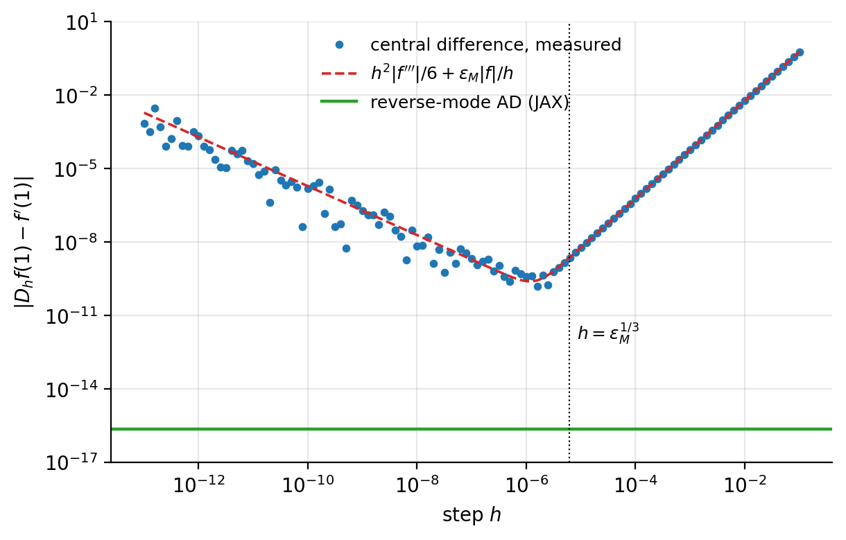
Figure 4.12: Absolute error of the central finite difference (4.73) for \(f(x)=\sin(2\pi x+x^{2})\) at \(x=1\), as a function of the step \(h\) (points), together with the model (4.75) (dashed): truncation error \(\propto h^{2}\) on the right, rounding error \(\propto1/h\) on the left, and a minimum of about \(10^{-10}\) near \(h\approx\epsilon_M^{1/3}\). The reverse-mode derivative computed by JAX has an error at the level of the unit roundoff, shown as the horizontal line, for any \(h\) because it involves no \(h\).
The transformations of JAX compose: jit(grad(f)) compiles the
gradient, vmap(grad(f)) vectorises it over a batch,
grad(grad(f)) differentiates it again and
jvp(grad(f),dots) gives Hessian–vector products. We shall use this
machinery freely from Chapter 5 onwards, and in
Chapter 8 we shall meet reverse mode again under its older name.
4.15. Practical tips#
The following advice is collected from the sources cited in this chapter and from experience; each item connects to something already derived.
Randomise the data when forming minibatches. Always shuffle before splitting into minibatches. Otherwise the ordering of the data becomes a systematic feature of the gradient sequence, and the method can fit spurious correlations arising purely from the order of presentation. If the data arrive sorted by class, an unshuffled minibatch may contain a single class and its gradient will point somewhere unhelpful.
Transform your inputs. Learning is difficult when the landscape mixes steep and flat directions, and Section The learning rate and the condition number made that statement quantitative: the iteration count scales with \(\kappa\). Standardising the inputs – subtracting the mean and dividing by the standard deviation, as in Section Arrays in practice: numpy, BLAS and LAPACK – equalises the scales and reduces \(\kappa\). Whenever possible, decorrelate the inputs as well. The reason is exactly Eq. (1.44): for a squared error cost the Hessian is the correlation matrix of the inputs, up to normalisation, so standardising and decorrelating make the landscape as close to spherical as it can be made, which by Eq. (4.26) is the best case. Since most deep networks are linear transformations followed by non-linearities, the intuition carries beyond the linear case; this is also the motivation for batch normalisation.
Monitor out-of-sample performance. Always track the cost on a validation set held out of training, as a proxy for the test set of Section Training error, test error and generalisation. When the validation error begins to rise while the training error still falls, the model has started to overfit and the run should be stopped. This early stopping improves performance substantially in many settings and costs nothing.
Adaptive methods do not always generalise well. As noted in Section Implementations, several studies have found that Adam, RMSProp and AdaGrad reach a worse test error than well-tuned SGD with momentum, particularly when the number of parameters exceeds the number of data points. It is not settled why adaptive methods train deep networks so effectively yet generalise less well; the practical conclusion is that a properly tuned SGD may match or beat them, and is worth trying.
Check your gradients. Before trusting an optimiser, verify the gradient it is given. Compare the analytical expression against a central finite difference,
with \(h\) around \(10^{-5}\), or against automatic differentiation. An optimiser given a wrong gradient does not usually crash; it quietly converges to the wrong answer, which is far harder to detect.
Do not compare learning rates across optimisers. Table 4.4 made the point: the same \(\gamma\) means different things to plain SGD and to Adam, because the latter has already normalised the gradient. Each method must be tuned on its own scale before any comparison is meaningful.
4.16. Summary and the programs#
The chapter has one argument, developed in stages.
Minimising a cost function is easy when the cost is convex, because by Section Convexity any stationary point is then a global minimum, and the least-squares and Ridge problems of Chapter 3 are convex. Newton’s method (4.8) solves such problems ideally, in a single step for a quadratic, and is invariant to how the parameters are scaled. It costs \(\bigO(p^{3})\) per step and is therefore unavailable for large models.
Gradient descent costs \(\bigO(p)\) and pays for it in iterations. The decoupled error recursion (4.19) explained exactly why: the step size is bounded above by \(2/\lambda_{\max}\) for stability while progress is governed by \(\lambda_{\min}\), so the iteration count scales with the condition number \(\kappa\) of the Hessian – and by Eq. (4.27) with the square of the condition number of the design matrix. This single number connects the chapter to the two before it: it is the quantity of Section Vector and matrix norms that governs numerical accuracy, the quantity of Section Statistical properties of the least-squares estimator that governs the variance of the fitted parameters, and now the quantity that governs how long training takes. Standardising features and adding a Ridge penalty improve all three at once.
The remedies then form a sequence, each recovering a little more of what Newton’s method has and gradient descent lacks. Momentum accumulates a discounted history of gradients, amplifying consistent directions by \(1/(1-\beta)\) and cancelling oscillatory ones, which improves the rate from \(\kappa\) to \(\sqrt{\kappa}\). Stochastic gradients replace the full sum by a minibatch – an unbiased estimate with noise \(\propto1/\sqrt{M}\), Eq. (4.43) – trading a worse rate per iteration for a far better rate per floating-point operation: by the count of Eq. (4.48) the statistical accuracy worth having is reached in a few passes over the data, where gradient descent needs \(\kappa\ln n\) of them, and Fig. 4.5 showed the factor to be two orders of magnitude on an ordinary problem. The price is that at a constant learning rate the iterate equilibrates in a cloud of radius \(\propto\sqrt{\gamma/M}\), Eq. (4.50), instead of converging, leaving the cost on a plateau \(\gamma\,\mathrm{tr}\,\bm{S}/(4M)\) that does not depend on the condition number, Eq. (4.51); the Robbins–Monro schedules, or an average over the iterates, repair this. Measured in epochs the batch size hardly matters, measured in seconds it matters a great deal (Table 4.3), and no comparison between optimisers means anything until the accuracy target and the horizontal axis have been stated. The adaptive methods are diagonal preconditioners, Eq. (4.57), that estimate the curvature from the second moment of the gradient: AdaGrad by an unbounded sum, which gives a built-in \(1/\sqrt{t}\) schedule and eventually stalls; RMSProp by an exponential moving average, which does not stall but cannot settle at a constant learning rate, Eq. (4.66); and Adam by combining RMSProp with momentum, whose averaging restores the ability to settle, and correcting the initialisation bias with the factors \(1-\beta_i^{t}\) derived in Eq. (4.69). Their learning rate is a trust region, Eq. (4.72), not a multiplier of the gradient; they are invariant to the scaling of individual features and blind to their correlation, Fig. 4.8.
The demonstration of Table 4.4 was deliberately unflattering, and its two lessons should be kept. A learning rate is not comparable across optimisers, because the adaptive methods have already normalised the gradient before \(\gamma\) multiplies it. And on a small, convex, well-conditioned problem the adaptive machinery buys nothing and can cost a great deal: these methods exist for large, ill-conditioned, non-convex landscapes, which is where we shall meet them from Chapter 5 onwards.
Finally, none of this is usable without gradients, and Section Automatic differentiation showed that they need not be derived by hand. Automatic differentiation applies the chain rule to the evaluation trace of a program: forward mode carries a tangent with every value and returns one Jacobian–vector product per sweep, reverse mode carries an adjoint with every node and returns one vector–Jacobian product per sweep, and by the cheap gradient principle of Proposition 4.2 the latter delivers the gradient with respect to all \(p\) parameters for the price of a few function evaluations, independent of \(p\). It is exact to rounding, where finite differences are limited to \(\epsilon_M^{2/3}\) by Eq. (4.76), and it is the reason the models of the later chapters can be written down at all.
The complete programs are collected in doc/BookML/BookPrograms:
gradient_descent.py– plain and momentum gradient descent on \(f(x)=x^{2}\) and on the least-squares and Ridge problems of Section Gradient descent for linear regression, with the analytical solutions for comparison, and the empirical verification of the stability bound (4.20) and the rate (4.26).stochastic_gradient.py– minibatch SGD with a varying number of batches, the time-decay schedule (4.52), the large-\(n\) comparison of Fig. 4.5 counted in floating-point operations, and the empirical check of the minibatch variance (4.43) and of the equilibration radius (4.50); the running mean of Section A worked example: the running mean and the practical loop with shuffled batches and early stopping of Section Learning rate schedules and stopping are separate listings, and the figure scriptBookFigures/ch04_sgd_figures.pyproduces Figs. 4.6 and 4.7, Table 4.3 and every number quoted in Section Stochastic gradient descent.adaptive_optimizers.py– AdaGrad, RMSProp and Adam as in Section Implementations, both as the epoch loop and as the step functionoptimiser_step, the learning-rate sweep of Table 4.4, the axis-aligned and rotated bowls of Fig. 4.8, and the same comparison repeated on a deliberately ill-conditioned design matrix.autodiff_examples.py– theDualclass of Section Forward mode: tangents and dual numbers and the two hand-worked examples of Section Two examples worked by hand, theautogradandJAXversions of the least-squares and Ridge gradients, the explicitjvp/vjpand Hessian–vector products of Section Automatic differentiation in Python: autograd and JAX, the four optimisers on the Rosenbrock function of Section The optimisers of this chapter on a non-convex function, and the finite-difference error curve of Fig. 4.12.
Each file runs as a script and reproduces the numbers quoted in this chapter. An executable version is available as a Jupyter notebook in the accompanying Jupyter-book.
4.17. Exercises#
4.17.1. Warm-up exercises#
Convexity from the definition. Show that \(f(x)=x^{2}\) is convex on \(\mathbb{R}\) using Eq. (4.1). Hint: show that \(\lambda f(x)+(1-\lambda)f(y)-f(\lambda x+(1-\lambda)y)\ge0\) for all \(x,y\) and \(\lambda\in[0,1]\).
Convexity from the second-order condition. Using the second-order condition of Section Convexity, show that (a) \(f(x)=e^{x}\) is convex on \(\mathbb{R}\); (b) \(g(x)=-\ln(x)\) is convex on \((0,\infty)\).
Compositions. Let \(f(x)=x^{2}\) and \(g(x)=e^{x}\). Show that \(f(g(x))\) and \(g(f(x))\) are convex on \(\mathbb{R}\). Show more generally that if \(f\) is any convex function then \(h(x)=e^{f(x)}\) is convex.
Norms are convex. A norm satisfies \(f(\alpha\bm{x})=|\alpha|f(\bm{x})\) and \(f(\bm{x}+\bm{y})\le f(\bm{x})+f(\bm{y})\). Using only these two properties and Eq. (4.1), show that a norm is convex. Deduce that both the Ridge and the Lasso cost functions of Chapter 3 are convex.
The stability bound (numerical). For the least-squares problem of Section Gradient descent for linear regression: (a) compute the eigenvalues of the Hessian (4.14) and hence \(\lambda_{\max}\), \(\lambda_{\min}\) and \(\kappa\); (b) run gradient descent for \(\gamma\) just below and just above \(2/\lambda_{\max}\) and confirm Eq. (4.20); (c) measure the number of iterations needed to reach a fixed accuracy for several \(\gamma\), and check that the minimum occurs near \(\gamma^{*}=2/(\lambda_{\max}+\lambda_{\min})\).
Conditioning and convergence (numerical). Construct design matrices with condition numbers \(\kappa_2(\bm{X})=10,10^{2},10^{3}\), for instance by rescaling the columns. (a) Measure the iteration count of gradient descent to fixed accuracy for each, and check the linear scaling with \(\kappa\) predicted by Eq. (4.26). (b) Repeat with momentum and verify the \(\sqrt{\kappa}\) scaling of Eq. (4.33). (c) Repeat after standardising the columns, and comment.
Momentum as a damped oscillator. Consider the one-dimensional quadratic \(C(\theta)=\tfrac{1}{2}\lambda\theta^{2}\). (a) Write the momentum update (4.28) as a two-term recurrence in \(\theta\). (b) Find the values of \(\gamma\) and \(\beta\) for which the recurrence has complex roots, and interpret them as oscillation. (c) Verify Eq. (4.32) numerically by applying momentum to a constant gradient.
Minibatch noise (numerical). For a fixed \(\bm{\theta}\), compute the minibatch gradient many times for batch sizes \(M=1,4,16,64\) and measure the standard deviation of its components. Verify the \(1/\sqrt{M}\) scaling predicted by Section The central limit theorem, and discuss what it implies about the cost of reducing gradient noise.
AdaGrad stalls (numerical). Reproduce the \(\gamma=0.01\) column of Table 4.4. (a) Plot the effective learning rate \(\gamma/\sqrt{r_{t,j}}\) against \(t\) for each coordinate and show that it decays towards zero. (b) Estimate the total distance the iterate can still travel after \(t\) steps, and compare with the distance remaining to the minimum. (c) Repeat with RMSProp and explain, using Eq. (4.65), why the decay does not occur.
Adam’s bias correction (numerical). (a) Implement Adam with and without the bias correction (4.70) and compare the first twenty steps. (b) For a constant gradient \(g\), verify Eq. (4.69) numerically. (c) Show that with \(\beta_2=0.999\) the uncorrected \(\sqrt{v_1}\) is smaller than the true root mean square gradient by a factor of about \(32\), and explain what that does to the first step.
Dual numbers. (a) Using only \(\varepsilon^{2}=0\), derive the rules for the quotient \((a+b\varepsilon)/(c+d\varepsilon)\) and for \(\sqrt{a+b\varepsilon}\), and check that they reproduce the quotient rule and \(d\sqrt{x}/dx\). (b) Show from Eq. (4.84) that dual numbers cannot deliver second derivatives, and that the “hyper-dual” algebra with two symbols \(\varepsilon_1,\varepsilon_2\), \(\varepsilon_1^{2}=\varepsilon_2^{2}=0\) but \(\varepsilon_1\varepsilon_2\neq0\), can. (c) Extend the
Dualclass of Section Forward mode: tangents and dual numbers withsqrtand__truediv__for a dual denominator, and verify your rules numerically.Forward and reverse sweeps by hand. For \(f(x_1,x_2)=x_1x_2+\exp(x_1x_2)-\sin x_1\) at \((x_1,x_2)=(1,2)\): (a) write down the evaluation trace and draw the computational graph, as in Eq. (4.78) and Fig. 4.10; (b) carry out the forward sweep (4.81) for both coordinate directions; (c) carry out the reverse sweep (4.87) once, and confirm that it delivers both partial derivatives; (d) count the multiplications in (b) and in (c), and check the operation count against Proposition 4.2.
Reverse mode for least squares. Write the least-squares cost (4.12) as the trace \(\bm{v}_1=\bm{X}\bm{\theta}\), \(\bm{v}_2=\bm{v}_1-\bm{y}\), \(v_3=\bm{v}_2^{T}\bm{v}_2/n\), with vector-valued nodes. Apply the reverse recursion (4.87) with the vector–Jacobian products (4.89) of each stage, and show that it produces the gradient (4.13) \(\frac{2}{n}\bm{X}^{T}(\bm{X}\bm{\theta}-\bm{y})\) without ever forming a Jacobian larger than \(\bm{X}\) itself. Explain why the adjoint \(\bar{\bm{v}}_1\) is what Chapter 8 will call the output error.
Hessian–vector products (numerical). (a) Implement Eq. (4.100) in JAX as forward-over-reverse,
jvp(grad(f)), and alternatively as reverse-over-reverse,grad(lambda x: grad(f)(x) @ v). Check both againstjax.hessianon the Ridge cost (4.16). (b) Use only Hessian–vector products and the conjugate-gradient method to solve the Newton system (4.8) for the Rosenbrock function (4.101), and reproduce the six-step convergence of Section The optimisers of this chapter on a non-convex function without ever forming the Hessian.The minibatch gradient as an estimator. (a) Derive Eq. (4.43) for sampling without replacement, starting from the fact that each example enters the batch with probability \(M/n\) and each pair with probability \(M(M-1)/(n(n-1))\). (b) On the least-squares problem of Section Gradient descent for linear regression, fix a point \(\bm{\theta}\), draw a few hundred minibatches for \(M=1,5,25\) and compare the mean and the standard deviation of the minibatch gradients with the full gradient and with Eq. (4.43). (c) Run SGD at a constant \(\gamma\) for \(M=5\) and \(M=20\), measure the size of the cloud in which the iterate settles along the flattest eigendirection, and compare with Eq. (4.50). (d) Derive the plateau (4.51) from Eq. (4.50), show that \(\mathrm{tr}\,\bm{S}\approx4\sigma^{2}p\) for least squares with standardised features, and verify both numerically. Why does the condition number drop out of the cost but not out of the distance \(\|\bm{\theta}-\hat{\bm{\theta}}\|\)?
The running mean. (a) Show by induction that the recursion (4.40) with \(\gamma_t=1/(t+1)\) makes \(\theta_t\) the mean of the first \(t\) samples. (b) Show that with a constant \(\gamma\) the iterate is an exponentially weighted average of the samples with stationary variance \(\gamma s_a^{2}/(2-\gamma)\), and check it numerically for \(\gamma=0.1\) and \(0.01\). (c) Replace the last iterate of (b) by the average of the iterates over the second half of the run and compare its error with that of (a).
Expected progress of one stochastic step. (a) Fill in the steps between the descent lemma and Eq. (4.44), stating where unbiasedness and where Eq. (4.42) are used. (b) For a quadratic cost the inequality is an equality if \(L\) is replaced by the appropriate Rayleigh quotients. On the least-squares problem of Section Gradient descent for linear regression, draw \(5000\) minibatches at a fixed \(\bm{\theta}\), measure the mean change of the cost and the fraction of steps that increase it, for \(M=1\), \(8\) and \(64\), far from the minimum and close to it. (c) Setting the progress and noise terms equal and using \(\|\nabla C\|^{2}\ge2\mu(C-C^{*})\) gives a bound on the plateau. Compare it with Eq. (4.51) and explain the factor \(\kappa\) by which the bound is pessimistic.
Counting flops. (a) Verify the count (4.38) and extend it to the Ridge gradient (4.17) and to one Newton step with the Hessian (4.14) formed and factorised. (b) For \(n=10^{6}\), \(p=10^{3}\), \(\kappa=10^{3}\) and \(M=64\), estimate from Eq. (4.48) the number of floating-point operations gradient descent, momentum and SGD need to reach the estimation error \(\sigma^{2}p/n\), and the number of epochs each corresponds to. (c) Repeat the experiment of Fig. 4.5 with \(n=10^{3}\) and with \(n=10^{6}\). Where does the crossover at which SGD overtakes gradient descent move, and why?
A fair comparison (numerical). Generate a least-squares problem with \(n=100\,000\), \(p=50\), correlated standardised features and controlled noise, and set aside a validation set. Compare gradient descent (tuned constant \(\gamma\)), SGD with \(M=1\) (decaying \(\gamma_t\)) and minibatch SGD with \(M=32\), \(128\) and \(512\) (tuned, constant and decaying), recording the training cost, the validation cost and the time. (a) Plot the validation cost against updates, examples processed, estimated floating-point operations and wall time, as in Fig. 4.7, with bands from at least five seeds. (b) Report, as in Table 4.3, what each method needs to reach the validation cost of the exact solution to within the estimation error (4.47). (c) Repeat for autoregressive correlations \(0\), \(0.5\), \(0.9\) and \(0.99\). How do the epoch counts of gradient descent and of SGD scale with \(\kappa\), and what does adding momentum change? (d) Replace the decaying schedule by a constant \(\gamma\) with iterate averaging over the second half of the run and place it in the table.
RMSProp cannot settle; Adam can. (a) For \(C=\frac12\lambda\theta^{2}\) with \(\lambda=1\), run RMSProp at \(\gamma=10^{-2}\) from \(\theta_0=1\) for \(10^{4}\) steps and plot \(|\theta_t|\). Confirm the limit cycle predicted by Eq. (4.66) and measure its amplitude for \(\gamma=10^{-1},10^{-2},10^{-3}\). (b) Repeat with Adam at the same \(\gamma\) and explain, using the first moment, why it converges. (c) Show from Eqs. (4.67)–(4.71) that the first Adam step is \(-\alpha\,\mathrm{sign}(\bm{g}_1)\), and that without bias correction it would be longer by \((1-\beta_1)/\sqrt{1-\beta_2}\). (d) Multiply one column of the design matrix of Section Gradient descent for linear regression by \(c=100\) and rerun gradient descent, Adam and AdaGrad from the same starting point. Which iteration counts change, and why?
The finite-difference error curve (numerical). Reproduce Fig. 4.12 for \(f(x)=e^{x}\) at \(x=1\) and for \(f(x)=\tan x\) at \(x=1.5\). From the measured minimum, estimate \(\epsilon_M\) and \(|f'''|\) using Eq. (4.76), and compare with the true values. Repeat in single precision (
np.float32) and explain the change.
4.17.2. Project-style exercise: optimisers on an ill-conditioned problem#
The comparison in Table 4.4 was made on a problem too easy to distinguish the methods. The purpose of this exercise is to build one that does, and thereby to see the arguments of this chapter operate.
Part a: build the landscape. Generate a polynomial regression problem from the Franke function of Section A complete example: the Franke function, or from a one-dimensional polynomial of degree ten with the Vandermonde design matrix (3.3). Compute \(\kappa_2(\bm{X})\) and \(\kappa_2(\bm{X}^{T}\bm{X})\) and confirm Eq. (4.27). Then produce a second version with the columns standardised and compare the two condition numbers.
Part b: plain gradient descent. Implement gradient descent with the analytical gradient (4.13). Determine empirically the largest stable \(\gamma\) and compare with Eq. (4.20). Plot the cost against iteration for several \(\gamma\) on both the raw and the standardised problem.
Part c: momentum and stochasticity. Add momentum and confirm the improvement in iteration count. Then implement minibatch SGD with the time-decay schedule (4.52), and compare convergence per iteration and per gradient evaluation. Which comparison is the fair one, and why?
Part d: the adaptive methods. Implement AdaGrad, RMSProp and Adam. For each, sweep \(\gamma\) over several orders of magnitude and record the best result; present the outcome as a table like Table 4.4. Discuss which methods are sensitive to \(\gamma\) and which are not, and relate your finding to whether the method normalises the gradient before applying \(\gamma\).
Part e: the diagonal approximation and its limits. Construct two problems with the same condition number, one whose Hessian is diagonal and one whose narrow valley runs at \(45\) degrees to the coordinate axes – the second is obtained from the first by an orthogonal rotation of the features, which by Section Orthogonal transformations leaves \(\kappa\) unchanged. Run all the methods on both. Explain, using the final notebox of Section Adam, why the adaptive methods help on the first and not on the second, and what this says about the difference between a diagonal approximation to \(\bm{H}\) and the real thing.
Part f: automatic differentiation.
Repeat part b using autograd or JAX instead of the
hand-derived gradient, and verify that the two agree to machine precision.
Then apply the gradient check (4.102) and compare the accuracy
of the finite difference with that of automatic differentiation as \(h\) is
varied over many orders of magnitude. Explain the shape of the resulting
curve using the discussion of round-off error in
Section Vector and matrix norms.