
2. Chapter 2: Elements of Probability Theory and Statistics#
Machine learning is inference from data, and data are noisy. Every number we compute from a finite sample – a mean, a fitted parameter, a test error – is itself a random quantity, and a result quoted without an estimate of its uncertainty is not a result. This chapter assembles the probability theory and statistics needed to make such statements precisely, in the order in which the rest of the book will need them.
The chapter has four parts. The first develops the language of probability: stochastic variables, distributions, expectation values, covariance, and the central limit theorem which explains why so much of statistics reduces to the Gaussian distribution. The second turns to estimators – the quantities we actually compute from a finite sample – and asks how far they can be trusted, including the awkward and frequently ignored case of correlated data. The third part is about assessing a model rather than a number: the split between training and test error, the bias-variance decomposition that explains why more complexity is not always better, and the resampling methods, bootstrap and cross-validation, that let us estimate generalisation error from the data we already have. The fourth part deals with generating randomness rather than analysing it: pseudo-random number generators, Markov chains and the Metropolis algorithm.
It is useful at the outset to distinguish two kinds of error. Statistical errors arise from the finiteness and randomness of the sample; they shrink, usually as \(1/\sqrt{n}\), as more data are collected, and they are what the machinery of this chapter is designed to quantify. Systematic errors arise from the method itself – a biased measurement, a model that cannot represent the truth, a preprocessing step that leaks information from the test set – and they do not shrink with more data. No amount of statistics will reveal a systematic error; only thinking about the method will. Much of the discipline of machine learning consists of converting what would otherwise be systematic errors into statistical ones.
2.1. Domains, stochastic variables and probability distributions#
Consider the tossing of two dice. The possible outcomes are
a set we call the domain, and to each element of the domain there corresponds a probability,
We cannot say in advance whether the next throw will give \(3\) or \(9\); that is what we mean by calling the outcome random. What we can say in advance is that each outcome has a definite probability. Recording a sequence of throws might give
in which the numbers of the domain appear in no predictable order but, over sufficiently many throws, in the predicted proportions.
A stochastic variable (or random variable) is thus characterised by two things: a domain containing all values it may assume, and a probability distribution over that domain. We write \(\mathbb{D}=\{x\}\) for the domain, so that \(X\in\mathbb{D}\), and reserve upper-case \(X\) for the variable and lower-case \(x\) for a particular value it takes.
Discrete and continuous distributions. In the discrete case the probability distribution function (PDF) \(p(x)\) gives the probability with which each value occurs,
In the continuous case \(p(x)\) does not itself give a probability – the probability of any single real number is zero – but a probability density: the probability that \(X\) lies in an infinitesimal interval around \(x\) is \(p(x)\,dx\), and the probability of landing in a finite interval is the integral
Qualitatively, a stochastic variable represents numbers drawn as if by chance from a specified PDF, in such a way that a large sample of them reproduces that PDF.
Closely related is the cumulative distribution function (CDF), the probability that \(X\) takes any value below \(x\),
Throughout this book we reserve the lower-case \(p\) for a density and the upper-case \(P\) for the corresponding cumulative function. The CDF is not merely bookkeeping: Section Random numbers shows that inverting it is the standard way of generating samples from an arbitrary distribution.
Properties every PDF must have. Two conditions are required. The first is positivity: a probability can be neither negative nor, in the discrete case, greater than one,
Note the asymmetry: a continuous density may perfectly well exceed unity, since only its integral is a probability. The second is normalisation – the probability that anything at all happens is one,
Table 2.1 collects these and the corresponding statements for the cumulative function.
Discrete PDF |
Continuous PDF |
|
|---|---|---|
Domain |
\(\{x_0,x_1,\dots,x_{N-1}\}\) |
\([a,b]\) |
Probability |
\(p(x_i)\) |
\(p(x)\,dx\) |
Cumulative |
\(P_i=\sum_{l=0}^{i}p(x_l)\) |
\(P(x)=\int_a^x p(t)\,dt\) |
Positivity |
\(0\le p(x_i)\le1\) |
\(p(x)\ge0\) |
Positivity |
\(0\le P_i\le1\) |
\(0\le P(x)\le1\) |
Monotonicity |
\(P_i\ge P_j\) if \(x_i\ge x_j\) |
\(P(x_i)\ge P(x_j)\) if \(x_i\ge x_j\) |
Normalisation |
\(P_{N-1}=1\) |
\(P(b)=1\) |
Table 2.1: Properties of discrete and continuous probability distribution functions and of the corresponding cumulative distributions.
2.2. Distributions we shall need#
A handful of distributions account for most of what happens in this book.
The uniform distribution. The simplest PDF assigns equal density to every point of an interval,
with \(\theta\) the Heaviside step function. For \(a=0\) and \(b=1\) this is simply \(p(x)\,dx=dx\) on \([0,1]\), which is what a random number generator produces and from which, as we shall see in Section Random numbers, every other distribution is obtained by transformation.
The Gaussian (normal) distribution. By far the most important continuous distribution is
with mean \(\mu\) and standard deviation \(\sigma\). For \(\mu=0\) and \(\sigma=1\) it is the standard normal distribution
and we write \(X\sim\mathcal{N}(\mu,\sigma^2)\) for a Gaussian variable. Its pre-eminence is not a matter of convenience: the central limit theorem of Section The central limit theorem shows that averages of almost anything become Gaussian, which is why Gaussian noise is the default assumption in regression and why the squared-error loss of Chapter 3 is the maximum-likelihood loss for that assumption.
The following code plots Eq. (2.7) for three parameter pairs.
import numpy as np
import matplotlib.pyplot as plt

x = np.linspace(-20.0, 20.0, 400)

for mu, sigma in [(0.0, 1.0), (1.0, 2.0), (2.0, 4.0)]:
    p = np.exp(-(x - mu)**2 / (2 * sigma**2)) / np.sqrt(2 * np.pi * sigma**2)
    plt.plot(x, p, label=rf"$\mu={mu}$, $\sigma={sigma}$")

plt.xlabel(r"$x$"); plt.ylabel(r"$p(x)$")
plt.legend(); plt.show()
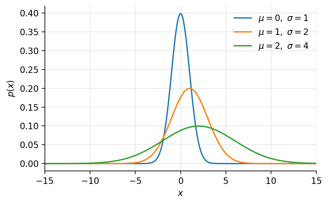
Figure 2.1: The Gaussian density (2.7) for three parameter pairs. Changing \(\mu\) translates the curve, changing \(\sigma\) both widens it and lowers its peak, the area remaining unity.
The multivariate Gaussian.
The generalisation to \(p\) correlated variables collected in a vector \(\bm{x}\in\mathbb{R}^{p}\) is
with \(\bm{\mu}\) the vector of means and \(\bm{\Sigma}\) the covariance matrix of Section The covariance matrix. Everything in Eq. (2.9) is linear algebra from Chapter 1: the exponent is a quadratic form, the normalisation involves a determinant computed from a Cholesky factorisation through Eq. (1.84), and the surfaces of constant density are ellipsoids whose axes are the eigenvectors of \(\bm{\Sigma}\) with lengths proportional to \(\sqrt{\lambda_i}\) – which is to say the principal components of Section Principal component analysis. Fitting Eq. (2.9) by maximum likelihood is what the derivative \(\partial\ln\Det{\bm{A}}/\partial\bm{A}\) of Eq. (1.49) was recorded for.
Other distributions. The exponential distribution
describes waiting times and appears whenever events occur independently at a constant rate. The binomial distribution
gives the probability of \(k\) successes in \(n\) independent trials each succeeding with probability \(q\); it is the distribution behind the logistic regression and binary classification of later chapters, and the quantity \(q\) is exactly what such a classifier estimates. Its limit for large \(n\) and small \(q\) at fixed \(nq=\lambda\) is the Poisson distribution \(p(k)=\lambda^{k}e^{-\lambda}/k!\), appropriate for counts of rare events.
2.3. Expectation values and moments#
Let \(h(x)\) be a function on the domain of a stochastic variable \(X\) with PDF \(p(x)\). The expectation value of \(h\) with respect to \(p\) is
with the integral replaced by a sum in the discrete case. Where the distribution is clear from the context we drop the subscript and write simply \(\mean{h}\); we shall also use the equivalent notation \(\mathbb{E}[h]\), which is more common in the machine learning literature and which we prefer when several distributions are in play at once.
A particularly useful class of expectation values are the moments
The zeroth moment \(\mean{1}\) is the normalisation condition (2.5). The first moment is the mean,
for the continuous and discrete cases respectively; qualitatively it is the centroid of the distribution.
The central moments are taken about the mean,
The zeroth and first are trivially \(1\) and \(0\). The second is the variance, and it is the quantity we shall use most,
The last line is worth memorising: the variance is the mean of the square minus the square of the mean. Its square root \(\sigma=\sqrt{\mean{(x-\mean{x})^2}}\) is the standard deviation, the root-mean-square deviation of the distribution from its mean, interpreted qualitatively as the spread of \(p\) about \(\mu\). Two properties follow immediately from the linearity of Eq. (2.12) and will be used repeatedly,
The variance is insensitive to a shift and scales with the square of a rescaling – which is the reason a feature measured in millimetres has a variance a million times larger than the same feature in metres, and hence the reason standardisation matters so much in Section Principal component analysis.
2.4. Covariance, correlation and independence#
Consider now a set \(\{X_i\}\) of \(n\) stochastic variables, not necessarily independent, with a joint PDF \(P(x_0,\dots,x_{n-1})\). The covariance of two of them is
with the marginal means
Expanding the product exactly as in Eq. (2.16) gives the computationally convenient form
of which Eq. (2.16) is the special case \(i=j\): the variance is the covariance of a variable with itself, \(\cov(X_i,X_i)=\var(X_i)\).
Collecting these numbers into a matrix \(\Sigma_{ij}=\cov(X_i,X_j)\) gives the covariance matrix, whose diagonal holds the variances. This is the population version of the sample covariance matrix already met in Section The covariance matrix, and everything proved there applies: it is symmetric, positive semi-definite, and its eigenvectors are the principal directions of the distribution.
Independence implies zero covariance. Two variables are independent if their joint PDF factorises, \(P(x_i,x_j)=p(x_i)p(x_j)\). In that case the expectation of the product factorises too, \(\mean{x_ix_j}=\mean{x_i}\mean{x_j}\), and Eq. (2.19) gives
The covariance matrix of independent variables is therefore diagonal.
The converse is false, and it matters
Zero covariance does not imply independence. Let \(X\) be symmetric about zero and put \(Y=X^{2}\); then \(\cov(X,Y)=\mean{x^3}-\mean{x}\mean{x^2}=0\) although \(Y\) is a deterministic function of \(X\). Covariance detects only linear dependence. Two consequences run through this book. First, principal component analysis produces uncorrelated components, not independent ones – which is precisely why independent component analysis exists as a separate method. Second, a correlation matrix showing nothing is not evidence that features carry no shared information; a neural network may still exploit a non-linear relationship that the covariance cannot see.
Correlation. Dividing by the two standard deviations makes the measure scale-free,
the bound being the Cauchy-Schwarz inequality (1.64) applied to the centred variables. The correlation matrix has unit diagonal, and it is what one should inspect when features carry different units.
The following code computes a covariance by hand and checks it against numpy.
import numpy as np

def covariance(x, y):
    """Sample covariance of two vectors, using the 1/n convention."""
    return np.mean((x - np.mean(x)) * (y - np.mean(y)))

rng = np.random.default_rng(2024)
n = 1000
x = rng.normal(size=n)
y = 4.0 + 3.0 * x + rng.normal(size=n)      # correlated with x by construction
z = rng.normal(size=n)                      # independent of both

print(covariance(x, y), covariance(x, z))
print(np.cov(np.vstack((x, y, z))))         # note: numpy uses 1/(n-1)
print(np.corrcoef(np.vstack((x, y, z))))    # the correlation matrix
Note the difference in convention: np.cov divides by \(n-1\) rather
than \(n\), for reasons explained in Section Samples, estimators and their properties.
2.5. The central limit theorem#
We can now state and derive the result that makes the Gaussian distribution inescapable. Suppose we draw values from some PDF \(p(x)\) and form the average of \(m\) of them,
and ask for the distribution \(\tilde{p}(z)\) of the new variable \(z\). The probability of obtaining a particular average is the product of the probabilities of the individual values, integrated over all combinations consistent with that average,
where the \(\delta\)-function enforces the constraint. The product form presupposes that the draws are independent, and this assumption is essential: everything in this section fails for correlated data, which is the subject of Section Correlated data and the autocorrelation function.
Carrying out the integral – most easily by writing the \(\delta\)-function as a Fourier integral, expanding the resulting characteristic function to second order in its argument, and letting \(m\) grow – yields the central limit theorem:
Central limit theorem
The PDF \(\tilde{p}(z)\) of the average of \(m\) independent values drawn from a distribution \(p(x)\) with mean \(\mu\) and finite variance \(\sigma^2\) tends, as \(m\) grows, to a Gaussian with mean \(\mu\) and variance \(\sigma^2/m\), whatever the shape of \(p(x)\).
The practical statement is the familiar one for the standard deviation of a mean,
usually called the standard error. Averaging four times as much data halves the uncertainty, and this square-root law is the reason large data sets help and the reason they help so slowly.
Two qualifications deserve emphasis, because both are routinely forgotten. The first is the requirement of a finite variance: distributions with heavy tails, such as the Cauchy distribution, have no finite \(\sigma^2\) and their sample means do not become Gaussian at all. The second is independence. When the values are correlated, Eq. (2.24) underestimates the true uncertainty, often by a large factor, and we take this up next.
Figure 2.2 illustrates both the theorem and its limits. Averages of uniform and of exponential variables become visibly Gaussian by \(m=10\) and are indistinguishable from it by \(m=100\), with the width shrinking as \(1/\sqrt{m}\); note that the exponential is strongly skewed and that the skew disappears nonetheless. The Cauchy distribution behaves entirely differently: its average is no better determined for \(m=100\) than for \(m=1\). The reason is that it has no finite variance, so the hypothesis of the theorem fails, and no amount of averaging helps. It is worth remembering that the central limit theorem is a statement with conditions and not a law of nature.
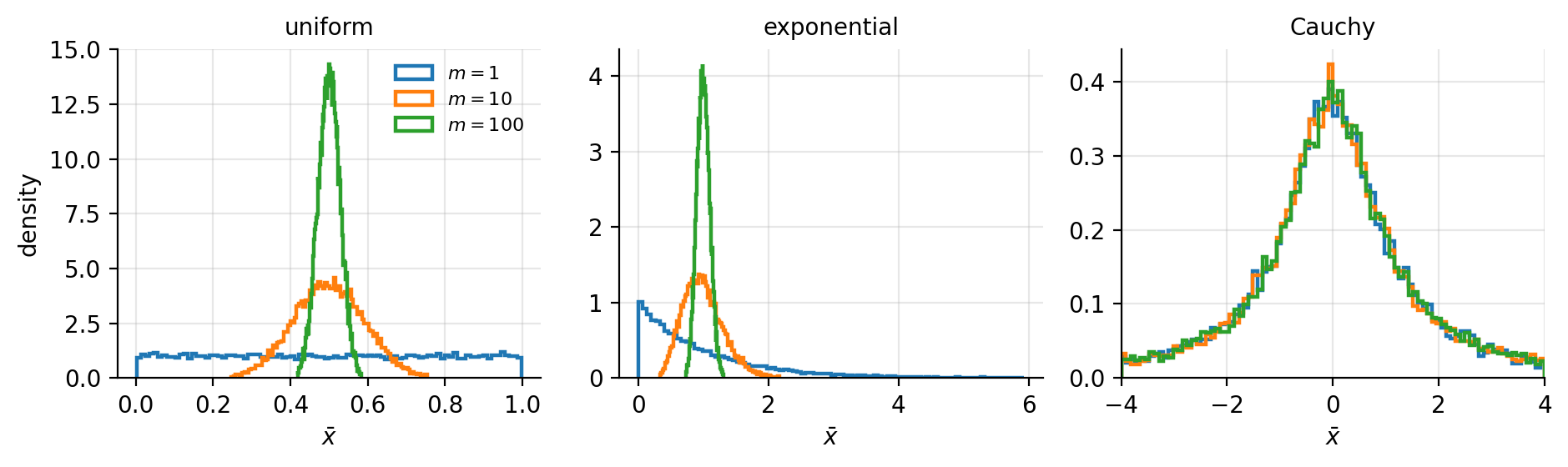
Figure 2.2: The central limit theorem at work, and failing. Histograms of the average of \(m\) independent draws for three distributions. Uniform and exponential averages converge to a Gaussian of width \(\sigma/\sqrt{m}\); Cauchy averages do not converge at all, the distribution of \(\bar{x}\) being independent of \(m\).
Machine learning connection
Equation (2.24) is why a test set of \(1000\) points gives a test error known to roughly \(3\%\) relative accuracy, and why comparing two models whose test errors differ by less than that is meaningless. It is also the theoretical justification for the bootstrap of Section Resampling: the jackknife and the bootstrap, and, applied to mini-batches, it explains why the gradient estimate in stochastic gradient descent has noise scaling as \(1/\sqrt{B}\) with batch size \(B\) – so that quadrupling the batch size only halves the gradient noise, at four times the cost per step.
2.6. Samples, estimators and their properties#
The framework of the preceding sections is idealised: it presumes we know \(p(x)\). In practice we have a finite set of measurements and must infer from them. A stochastic process produces a chain of values \(\{x_0,x_1,\dots\}\); we call these our measurements and the whole set our sample, and we assume they are distributed according to some unknown PDF \(p_X(x)\). Rather than determine \(p_X\) in full, we usually want only its lowest moments.
For a sample of size \(n\) the sample mean and sample variance are
These are estimators: functions of the data, used to approximate properties of the underlying distribution. Being functions of random variables, estimators are themselves random variables, with distributions of their own. This observation is the foundation of everything that follows, and in particular of the resampling methods of Sections Resampling: the jackknife and the bootstrap and Cross-validation, whose entire purpose is to explore that distribution numerically.
Bias, variance and mean squared error. Let \(\hat{\theta}\) be an estimator of a quantity \(\theta\). Its bias is
the systematic part of the error, and an estimator with zero bias is called unbiased. Its variance \(\var(\hat{\theta})\) measures how much it moves when the sample is redrawn. The two combine into the mean squared error, by adding and subtracting \(\mathbb{E}[\hat{\theta}]\),
the cross term vanishing because \(\mathbb{E}[\hat{\theta}-\mathbb{E}[\hat{\theta}]]=0\). Equation (2.27) is the bias-variance decomposition in its simplest form, and Section The bias-variance tradeoff is nothing but this identity applied to a prediction rather than a parameter. It already carries the central lesson: an unbiased estimator is not automatically a good one, since a biased estimator with much smaller variance can have the smaller total error. Ridge regression, introduced in Eq. (1.42) and analysed in Chapter 3, is exactly such a trade.
An estimator is consistent if it converges in probability to \(\theta\) as \(n\to\infty\), which by Eq. (2.27) follows if both bias and variance vanish in that limit.
Why \(n-1\). The sample mean is unbiased, \(\mathbb{E}[\bar{x}]=\mu\), directly from the linearity (2.17). The variance is more subtle. Using \(\bar{x}\) in place of the unknown \(\mu\) makes the sum of squared deviations systematically too small, because \(\bar{x}\) is the value that minimises that sum for the given sample. One data point has been spent estimating the mean, and a short calculation shows
so dividing by \(n-1\) rather than \(n\) restores unbiasedness. This is
Bessel’s correction, and it is why np.cov and np.std
differ in their default ddof settings – a discrepancy that matters
for small samples and is irrelevant for large ones.
Repeated experiments. It is often natural to think of a sample as one of several repetitions of an experiment. Suppose an experiment yielding \(n\) measurements is repeated \(m\) times, giving values \(x_{\alpha,k}\) with \(\alpha=1,\dots,m\) and \(k=1,\dots,n\). The total average is
and the variance of that average is
while the sample variance over all \(mn\) individual measurements is
These are experimental quantities and may differ, sometimes considerably, from the exact \(\mu_X\), \(\var(X)\) and \(\cov(X,Y)\) they estimate. The relation between Eqs. (2.30) and (2.31) is the subject of the next section.
2.7. Correlated data and the autocorrelation function#
Equation (2.30) contains a double sum over \(k\) and \(l\). Separating the diagonal terms \(k=l\) from the rest gives
in which the first term is the sample variance divided by \(n\) – exactly the central limit result (2.24) – and the second is a sum of covariances between distinct measurements. If the measurements are uncorrelated the second term vanishes and Eq. (2.24) is recovered. If they are correlated it does not, and the naive standard error is wrong.
The first term is cheap: we need only accumulate running sums of \(x\) and \(x^2\). The correlation term is expensive, since it requires every pair and therefore the storage of all measurements until the end. To organise it, group the pairs by their separation \(d=l-k\),
so that the correlation term becomes \(2\sum_{d=1}^{n-1}f_d/n\) and
The quantity \(f_d\) measures the correlation between measurements separated by \(d\) steps, and \(f_0=\sigma^2\) by construction. Normalising by the variance defines the autocorrelation function
in terms of which Eq. (2.34) takes the compact form
The factor \(\tau\) is the autocorrelation time. For independent data \(\tau=1\) and we recover Eq. (2.24); for correlated data \(\tau>1\), and the effective number of independent measurements is not \(n\) but \(n/\tau\). Ignoring this is one of the most common ways of quoting an error bar that is too small by an order of magnitude.
Figure 2.3 shows the effect for a first-order autoregressive sequence, \(x_{t+1}=\phi x_t+\eta_t\), which decays as \(\kappa_d=\phi^{d}\) and for which the correlation time can be computed exactly, \(\tau=(1+\phi)/(1-\phi)\). With \(\phi=0.9\) this gives \(\tau=19\): the effective number of independent measurements is one nineteenth of the number recorded, and an error bar computed from Eq. (2.24) is too small by a factor of \(\sqrt{19}\approx4.4\).
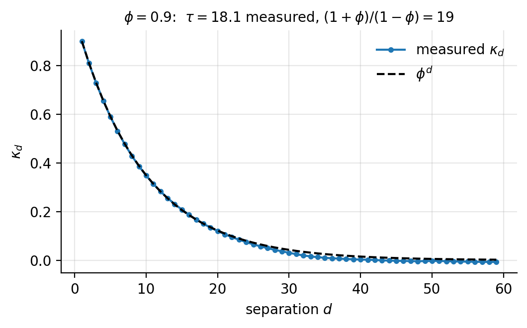
Figure 2.3: Autocorrelation function (2.35) of an autoregressive sequence with \(\phi=0.9\), compared with the exact \(\phi^{d}\). The measured correlation time agrees with the prediction \((1+\phi)/(1-\phi)\).
Machine learning connection
Correlated samples are the rule rather than the exception. Successive states of a Markov chain (Section Markov chains and the Metropolis algorithm) are correlated by construction, so any expectation value estimated from a Metropolis run needs Eq. (2.36) rather than Eq. (2.24). Time series – prices, sensor readings, patient records – are correlated, which is why splitting them randomly into training and test sets is a serious error: a randomly chosen test point sits between two training points that are nearly identical to it, and the test error measures interpolation rather than prediction. The same applies to data with group structure, such as several images of the same patient; the split must then respect the groups. A test error computed on correlated data is optimistic for the same reason that Eq. (2.24) is optimistic.
2.8. The statistics of the least-squares estimator#
The general theory above becomes concrete when applied to the estimator we already derived in Chapter 1. Assume the data are generated by a linear model with additive noise,
with the errors independent,
so that the noise covariance matrix is \(\sigma^2\bm{I}_{nn}\). Here \(\bm{X}\) is the fixed \(n\times p\) design matrix of Eq. (1.1) and \(\bm{\theta}\) the true parameter vector. The randomness of \(\bm{\varepsilon}\) makes \(\bm{y}\) random too: since \(\bm{X}_{i,\ast}\bm{\theta}\) is a non-random scalar,
where \(\bm{X}_{i,\ast}\) denotes row \(i\) of the design matrix. This is the first place in the book where a random and a non-random quantity are added, and since every statistical statement about regression rests on the distinction, it is worth being precise about what it means and why Eq. (2.39) follows from it.
What is random here, and what is not.
Equation (2.37) contains four objects, and only one of them is stochastic. The noise \(\bm{\varepsilon}\) is a random vector: it takes a different value every time the experiment is repeated, and those values follow the distribution (2.38). The parameter vector \(\bm{\theta}\) is a set of fixed numbers – unknown to us, which is the whole problem, but not random; nature does not redraw it between measurements. The design matrix \(\bm{X}\) is likewise treated as a fixed array of numbers: the inputs \(\bm{x}_i\) at which the measurements were taken are regarded as chosen, or at least as given, and the analysis is carried out for those inputs. Statisticians call this the fixed design viewpoint, and everything in this section is conditional on the observed \(\bm{X}\). And the function \(f\) that the model is trying to capture is a non-stochastic, or deterministic, function: a fixed rule that returns the same value \(f(\bm{x})\) every time it is evaluated at the same input. Nothing about \(f\) changes from one repetition of the experiment to the next; what changes is the noise added to it. If we could measure the response at the same \(\bm{x}_i\) a thousand times, the thousand values of \(y_i\) would scatter about the single fixed number \(f(\bm{x}_i)\), and the scatter would be entirely that of \(\varepsilon_i\).
A non-random quantity \(c\) can be accommodated in the formalism of Section Expectation values and moments by regarding it as a stochastic variable whose distribution is concentrated at a single point, \(p(c')=\delta(c'-c)\) with \(\delta\) the Dirac delta function. Inserting this into the definition (2.12) gives
the expectation of a constant is the constant, and a constant has no variance. These two lines are all that “non-random” means for the purposes of computing moments.
Deriving Eq. (2.39). Write \(\mu_i=\bm{X}_{i,\ast}\bm{\theta}=\sum_j X_{ij}\theta_j\) for the \(i\)th fitted value at the true parameters. It is a sum of products of fixed numbers and is therefore itself a fixed number, and the model says \(y_i=\mu_i+\varepsilon_i\). Because \(\mu_i\) is a constant, the distribution of \(y_i\) is that of \(\varepsilon_i\) shifted by \(\mu_i\): if \(p_\varepsilon\) is the noise density, \(p(y_i)=p_\varepsilon(y_i-\mu_i)\). The expectation then follows directly from the definition (2.12) by the substitution \(e=y_i-\mu_i\),
where the first integral is the normalisation (2.5) and the second vanishes because the noise has zero mean. The variance follows from the central moment (2.15) by the same substitution,
Both results are the rule (2.17) with \(a=1\) and \(b=\mu_i\): adding a constant shifts the mean by that constant and leaves the variance untouched, because the variance measures spread about the mean and a constant shift moves the mean and every value together. The same argument applied to two different observations gives \(\cov(y_i,y_j)=\mathbb{E}[(y_i-\mu_i)(y_j-\mu_j)] =\mathbb{E}[\varepsilon_i\varepsilon_j]=\cov(\varepsilon_i,\varepsilon_j)\), so the whole vector satisfies
the observations inherit the covariance structure of the noise exactly, and the deterministic part of the model contributes only to the mean. When the noise is Gaussian, \(\bm{y}\) is the multivariate Gaussian (2.9) with \(\bm{\mu}=\bm{X}\bm{\theta}\) and \(\bm{\Sigma}=\sigma^{2}\bm{I}\), which is the form the likelihood of Chapter 3 will take.
A short simulation makes the statement concrete. The design and the parameters are fixed once; only the noise is redrawn, a hundred thousand times; and the sample mean and variance of each \(y_i\) over the repetitions are compared with Eq. (2.39).
import numpy as np

rng = np.random.default_rng(2024)
x = np.linspace(0.0, 1.0, 5)            # the design is fixed once and for all
X = np.column_stack([np.ones_like(x), x, x**2])
theta, sigma = np.array([1.0, -2.0, 3.0]), 0.5
mu = X @ theta                          # non-random: the same in every repetition

Y = mu + sigma * rng.normal(size=(100000, len(x)))  # 100000 draws of the noise only
print("X theta        :", np.round(mu, 3))
print("mean of y      :", np.round(Y.mean(axis=0), 3))
print("variance of y  :", np.round(Y.var(axis=0), 3), "  sigma^2 =", sigma**2)
print("cov(y_0, y_1)  :", np.round(np.cov(Y[:, 0], Y[:, 1])[0, 1], 4))
X theta        : [1.    0.688 0.75  1.188 2.   ]
mean of y      : [1.    0.686 0.751 1.188 2.   ]
variance of y  : [0.251 0.252 0.252 0.251 0.249]   sigma^2 = 0.25
cov(y_0, y_1)  : 0.0015
The means agree with \(\bm{X}\bm{\theta}\) to the third decimal, the variances
with \(\sigma^{2}\), and the covariance between two observations is zero to
within the sampling error of Eq. (2.24). Note what was
not redrawn: the array X is the same object in all hundred
thousand repetitions, which is exactly what the fixed-design assumption
says.
The model as an approximation of \(f\). Equation (2.37) asserts more than that \(f\) is non-stochastic: it asserts that \(f\) is linear in the features, so that \(f(\bm{x}_i)=\bm{X}_{i,\ast}\bm{\theta}\) exactly, for some \(\bm{\theta}\). The two assumptions are independent and it is worth separating them. Suppose only the weaker one holds, so that the data are generated by \(y_i=f(\bm{x}_i)+\varepsilon_i\) with \(f\) a fixed but otherwise arbitrary function. Nothing in the derivation of Eqs. (2.41) and (2.42) used the form of \(\mu_i\), only that it was a constant, so the conclusion survives unchanged with \(\mu_i=f(\bm{x}_i)\):
This is the sense in which the linear model \(\bm{X}\bm{\theta}\) approximates \(f\): it is a candidate for the deterministic part of the data, the mean of \(\bm{y}\), and the noise variance is untouched by how good or bad the candidate is. If \(f\) really is linear in the features, Eq. (2.44) reduces to Eq. (2.39) and the estimator below is unbiased. If it is not, then no choice of \(\bm{\theta}\) makes \(\bm{X}_{i,\ast}\bm{\theta}\) equal to \(f(\bm{x}_i)\) at every \(i\), and the discrepancy \(f(\bm{x}_i)-\bm{X}_{i,\ast}\bm{\theta}\) is a fixed number, not a random one: it does not average away with more data, it is invisible in the residuals, whose scatter still has variance \(\sigma^{2}\), and it reappears as the squared-bias term of Section The bias-variance tradeoff. A deterministic \(f\) that the model cannot represent is thus the source of bias, exactly as the random \(\bm{\varepsilon}\) is the source of variance; keeping the two apart is what the decomposition of that section is for.
Machine learning connection
The fixed-design viewpoint is the natural one for a designed experiment, where the inputs are chosen by the experimenter. In machine learning the inputs are usually themselves a random sample – the pixels of whichever images happened to be collected – and one speaks of a random design. The two viewpoints are reconciled by conditioning: every expectation in this section is \(\mathbb{E}[\,\cdot\,|\,\bm{X}]\), an average over the noise for the inputs actually observed, and the results hold as stated for every \(\bm{X}\) that might have been drawn. The bias-variance decomposition of Section The bias-variance tradeoff averages over training sets, inputs included, and the bootstrap that estimates it resamples whole rows \((\bm{x}_i,y_i)\) rather than the noise alone; the reader should keep in mind which expectation is meant when a result from one setting is quoted in the other.
The estimator is unbiased. The least-squares estimator of Eq. (1.39) is \(\hat{\bm{\theta}}=(\bm{X}^{T}\bm{X})^{-1}\bm{X}^{T}\bm{y}\). Taking its expectation and using \(\mathbb{E}[\bm{y}]=\bm{X}\bm{\theta}\),
so ordinary least squares is unbiased, provided the model (2.37) is correct. That proviso carries all the weight: if the true \(f(\bm{x})\) is not linear in the features, the estimator is biased no matter how much data we collect, and that bias is the first term of the decomposition in Section The bias-variance tradeoff.
The variance. Writing \(\bm{A}=(\bm{X}^{T}\bm{X})^{-1}\bm{X}^{T}\) so that \(\hat{\bm{\theta}}=\bm{A}\bm{y}\), and using \(\mathbb{E}[\bm{y}\bm{y}^{T}]=\bm{X}\bm{\theta}\bm{\theta}^{T}\bm{X}^{T} +\sigma^2\bm{I}_{nn}\),
that is
This is the result promised in Section The Hessian matrix: the covariance matrix of the fitted parameters is the inverse Hessian (1.44) scaled by the noise variance. The standard error of the \(j\)th coefficient is the square root of the corresponding diagonal element,
from which a confidence interval follows in the usual way, and in practice \(\sigma^2\) is itself estimated from the residuals as \(\hat{\sigma}^2=\|\bm{y}-\bm{X}\hat{\bm{\theta}}\|_2^2/(n-p)\), the divisor \(n-p\) being Bessel’s correction (2.28) generalised to \(p\) fitted parameters.
Machine learning connection
Read Eq. (2.47) through the singular value decomposition. By Eq. (1.115), \((\bm{X}^{T}\bm{X})^{-1}=\bm{V}\tilde{\bm{\Sigma}}^{-2}\bm{V}^{T}\), so the variance along the \(i\)th right singular direction is \(\sigma^2/\sigma_i^2\). A small singular value – near-collinear features – produces an enormous variance in that direction, which is the statistical statement of the numerical warning given in Section Rank, the pseudoinverse and ill-conditioned design matrices. The ill-conditioning we diagnosed there as a loss of significant digits is here diagnosed as an inability of the data to determine the parameter. Both readings describe the same fact, and both are repaired by the same shrinkage: Ridge regression trades the unbiasedness (2.45) for a variance reduced by the factors of Eq. (1.130), a bargain which Eq. (2.27) tells us is worth taking whenever the squared bias introduced is smaller than the variance removed.
2.9. Training error, test error and generalisation#
Up to this point we have asked how accurately a number is determined. We now ask a different question: how well will a fitted model perform on data it has never seen? This is the question of generalisation, and it cannot be answered by looking at the data used for fitting.
The standard measure for continuous predictions is the mean squared error of Eq. (1.33); the mean absolute error is an alternative, less sensitive to outliers, corresponding to the \(1\)-norm rather than the \(2\)-norm in the sense of Section Vector and matrix norms. Whichever loss is chosen, we must distinguish two quantities:
the training error \(\mathrm{Err}_{\mathrm{Train}}\), the average loss over the data used to fit the model;
the test error or prediction error \(\mathrm{Err}_{\mathrm{Test}}\), the average loss on data held out from fitting entirely.
Only the second estimates generalisation. The first can always be driven to zero by a sufficiently flexible model – a polynomial of degree \(n-1\) passes exactly through \(n\) points – and a model that has done so has memorised the sample rather than learned the process behind it.
As model complexity grows, the training error decreases monotonically and saturates near zero. The test error behaves differently: it falls at first, as the model becomes able to represent genuine structure, reaches a minimum, and then rises again as the model begins to fit the noise. The location of that minimum is what model selection seeks, and the shape of the curve is explained by the decomposition of the next section.
Machine learning connection
A test set is only a test set as long as it has been used once. Every time a hyperparameter is tuned by looking at the test error, information leaks from the test set into the model, and the test error becomes an optimistic estimate of generalisation – a systematic error in the sense of the introduction to this chapter, invisible to any of the statistics of this chapter. The standard discipline is a three-way split: train on one part, select hyperparameters on a validation part, and touch the test part exactly once, at the end. When data are scarce, the cross-validation of Section Cross-validation replaces the validation set. The same warning applies to preprocessing: as noted in Section Arrays in practice: numpy, BLAS and LAPACK, means and standard deviations used for scaling must be computed on the training part alone.
2.10. The bias-variance tradeoff#
We now derive the decomposition that governs the shape of the test-error curve. The argument is a direct application of Eq. (2.27), with the estimator being a prediction rather than a parameter. It is stated here for continuous predictions, but the intuition carries over to classification.
Let the data be generated by a noisy process,
with \(f\) the unknown true function and the noise of zero mean and variance \(\sigma^{2}\). We fit a model on a training set drawn at random, obtaining predictions \(\tilde{\bm{y}}\), and we ask for the expected squared error on a test point. The expectation is taken over the randomness of the training set and of the noise; this is the essential point, and the source of most confusion about the result. The model \(\tilde{\bm{y}}\) is a random variable because the data it was fitted to were random.
The cost we wish to decompose is
Insert Eq. (2.49) and add and subtract \(\mathbb{E}[\tilde{\bm{y}}]\), the average prediction over training sets,
Expanding the square produces three squared terms and three cross terms. The cross terms all vanish: those involving \(\bm{\varepsilon}\) because the noise has zero mean and is independent of the training set, and the remaining one because \(\mathbb{E}[\tilde{\bm{y}}-\mathbb{E}[\tilde{\bm{y}}]]=0\) while \(\bm{f}\) is not stochastic. What survives is
The three terms have distinct meanings.
The bias measures how far the average prediction is from the truth. It is the error caused by the simplifying assumptions built into the model: a straight line fitted to curved data has a large bias, and no quantity of data will remove it.
The variance measures how much the prediction moves when the training set is redrawn. A flexible model chases the noise in whatever sample it is given, so its predictions differ substantially from one training set to the next, even though it may be unbiased on average.
The irreducible error \(\sigma^{2}\) is the variance of the noise itself. No model, however good, can predict a random term, so \(\sigma^{2}\) is a floor beneath the test error. A model whose test error is at or below \(\sigma^{2}\) is not excellent; it has leaked test data or the noise estimate is wrong.
Increasing model complexity decreases the bias and increases the variance. The test error, being their sum plus a constant, has a minimum somewhere in between, and finding it is the entire business of model selection.
Estimating the three terms. Equation (2.52) involves an expectation over training sets, which in practice we do not have – we have one data set. The bootstrap of Section Resampling: the jackknife and the bootstrap manufactures the missing ensemble by resampling, and the following code uses it to compute all three terms for a polynomial fit of fixed degree.
import numpy as np
from sklearn.linear_model import LinearRegression
from sklearn.preprocessing import PolynomialFeatures
from sklearn.model_selection import train_test_split
from sklearn.pipeline import make_pipeline
from sklearn.utils import resample

np.random.seed(2018)

n, n_bootstraps, degree = 500, 100, 18      # a deliberately high degree
x = np.linspace(-1, 3, n).reshape(-1, 1)
y = np.exp(-x**2) + 1.5 * np.exp(-(x - 2)**2) + np.random.normal(0, 0.1, x.shape)

x_train, x_test, y_train, y_test = train_test_split(x, y, test_size=0.2)
model = make_pipeline(PolynomialFeatures(degree=degree),
                      LinearRegression(fit_intercept=False))

# Column i holds the predictions of the model fitted to bootstrap sample i
y_pred = np.empty((y_test.shape[0], n_bootstraps))
for i in range(n_bootstraps):
    x_, y_ = resample(x_train, y_train)
    y_pred[:, i] = model.fit(x_, y_).predict(x_test).ravel()

# Expectations over training sets are averages along axis 1; keepdims=True
# preserves the column shape and is essential for the bias to come out right.
error    = np.mean(np.mean((y_test - y_pred)**2, axis=1, keepdims=True))
bias     = np.mean((y_test - np.mean(y_pred, axis=1, keepdims=True))**2)
variance = np.mean(np.var(y_pred, axis=1, keepdims=True))

print(f"Error = {error:.5f}, Bias^2 = {bias:.5f}, Var = {variance:.5f}")
print(f"{error:.5f} >= {bias:.5f} + {variance:.5f} = {bias + variance:.5f}")
Note that the bias computed this way absorbs the irreducible error, since \(y_{\mathrm{test}}\) rather than the unknown \(f\) appears in it; the printed identity is therefore an inequality. Sweeping the polynomial degree traces out the whole trade-off:
import matplotlib.pyplot as plt

n, n_bootstraps, maxdegree = 40, 100, 14
x = np.linspace(-3, 3, n).reshape(-1, 1)
y = np.exp(-x**2) + 1.5 * np.exp(-(x - 2)**2) + np.random.normal(0, 0.1, x.shape)
x_train, x_test, y_train, y_test = train_test_split(x, y, test_size=0.2)

error    = np.zeros(maxdegree)
bias     = np.zeros(maxdegree)
variance = np.zeros(maxdegree)

for degree in range(maxdegree):
    model = make_pipeline(PolynomialFeatures(degree=degree),
                          LinearRegression(fit_intercept=False))
    y_pred = np.empty((y_test.shape[0], n_bootstraps))
    for i in range(n_bootstraps):
        x_, y_ = resample(x_train, y_train)
        y_pred[:, i] = model.fit(x_, y_).predict(x_test).ravel()

    error[degree]    = np.mean(np.mean((y_test - y_pred)**2, axis=1, keepdims=True))
    bias[degree]     = np.mean((y_test - np.mean(y_pred, axis=1, keepdims=True))**2)
    variance[degree] = np.mean(np.var(y_pred, axis=1, keepdims=True))

plt.plot(range(maxdegree), error,    label="Error")
plt.plot(range(maxdegree), bias,     label="Bias$^2$")
plt.plot(range(maxdegree), variance, label="Variance")
plt.xlabel("Polynomial degree"); plt.legend(); plt.show()
The resulting figure is the canonical one: the bias falls steeply and flattens, the variance is negligible at low degree and grows without bound, and their sum has a clear minimum.
Figure 2.4 is that figure. Three features are worth naming. The squared bias falls by two orders of magnitude between degrees zero and four and then flattens: beyond degree four the polynomial family is rich enough to represent the underlying function, and additional flexibility buys no reduction in bias. The variance is negligible at low degree and then grows steadily, since a more flexible model chases the noise in whichever bootstrap sample it is given. Their sum, the test error, therefore falls, reaches a minimum around degree four or five, and rises thereafter. Model selection is the business of locating that minimum, and Section Cross-validation is how it is done without a test set.
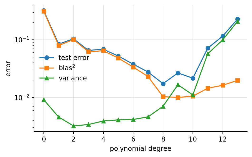
Figure 2.4: The bias-variance decomposition (2.52) for a polynomial fit, with the three terms estimated by the bootstrap. Bias falls and saturates, variance grows without limit, and the test error has a minimum in between.
Machine learning connection
Every regularisation method in this book is a deliberate move along this curve. Ridge and Lasso add bias in order to remove variance; early stopping halts training before the variance has grown; dropout and data augmentation reduce variance in neural networks; bagging and random forests average many high-variance models to cancel their variance while leaving the bias untouched, whereas boosting reduces bias by combining many high-bias models. Knowing which of the two terms a method attacks is often enough to predict whether it will help on a given problem. It should be added that the clean picture above is a statement about models of moderate capacity; the double-descent behaviour observed in heavily overparameterised networks shows that the test error can fall again beyond the interpolation threshold, and we return to this in the chapter on neural networks.
2.11. Resampling: the jackknife and the bootstrap#
Since \(\hat{\theta}=\hat{\theta}(\bm{X})\) is a function of random variables, it is itself a random variable with some PDF \(p(t)\). If we knew \(p(x)\), the distribution generating the data, we could learn everything about \(p(t)\) by brute force: draw a fresh sample \((x_0^{*},\dots,x_{n-1}^{*})\) from \(p(x)\), compute a replica \(\hat{\theta}^{*}\), repeat many times, and histogram the results. The difficulty is that \(p(x)\) is exactly what we do not know.
Efron’s idea. In 1979 Efron asked what happens if we replace \(p(x)\) by the empirical distribution – the relative frequency of the observations we actually have. If we draw new samples in accordance with the observed frequencies, do we recover the right answer in an asymptotic sense? The answer is yes, and drawing from the empirical distribution is nothing more than drawing from the observed values with replacement.
The independent bootstrap therefore works as follows:
Draw with replacement \(n\) values from the observations \(\bm{x}=(x_0,\dots,x_{n-1})\), forming a resample \(\bm{x}^{*}\).
Evaluate the estimator on the resample to obtain \(\hat{\theta}^{*}\).
Repeat \(k\) times.
The relative frequency of the \(k\) values \(\hat{\theta}^{*}\) estimates \(p(t)\). In practice one never draws the histogram; one simply applies the estimator of interest to the collection, using for instance the sample variance (2.25) of the \(\hat{\theta}^{*}\) as an estimate of \(\var(\hat{\theta})\).
The central limit theorem of Section The central limit theorem is what makes this work: the bootstrap distribution of a mean-like statistic approaches the same Gaussian as the true sampling distribution. It also marks the limits of the method. The bootstrap assumes independent, identically distributed observations; for correlated data it fails, for the reason discussed in Section Correlated data and the autocorrelation function, and variants such as the block bootstrap exist precisely to repair this.
The bootstrap is attractive because it is general: it requires no distributional assumption such as Gaussian errors, it applies to statistics whose sampling distributions are difficult or impossible to derive analytically, it copes with complicated sampling designs, and it is often more accurate than asymptotic formulae when the sample is small. It should be said that when the data are independent and identically distributed and all we want is the variance of a mean, Eq. (2.24) already answers the question and no bootstrap is needed.
The jackknife. The older jackknife is a special case. Instead of resampling, it systematically leaves out one observation at a time. Writing
for the sample with observation \(i\) removed, and \(\hat{\theta}_i\) for the estimator computed on it, the spread of the \(n\) values \(\hat{\theta}_i\) estimates the variance of \(\hat{\theta}\) and their mean gives a bias estimate. Both jackknife and bootstrap require independent, identically distributed variables and both fail without that assumption.
import numpy as np

def bootstrap(data, statistic, k=1000, rng=None):
    """Bootstrap estimate of the distribution of a statistic."""
    rng = np.random.default_rng() if rng is None else rng
    n = len(data)
    replicas = np.empty(k)
    for i in range(k):
        sample = data[rng.integers(0, n, n)]      # draw n values with replacement
        replicas[i] = statistic(sample)
    return replicas


def jackknife(data, statistic):
    """Leave-one-out replicas of a statistic."""
    n = len(data)
    return np.array([statistic(np.delete(data, i)) for i in range(n)])


rng = np.random.default_rng(2024)
mu, sigma, n = 100.0, 15.0, 10000
x = rng.normal(mu, sigma, n)

t = bootstrap(x, np.mean, k=1000, rng=rng)
print(f"original {np.mean(x):.5f}  bootstrap mean {np.mean(t):.5f}"
      f"  std. error {np.std(t):.5f}")
print(f"central limit theorem prediction: {np.std(x) / np.sqrt(n):.5f}")

tj = jackknife(x, np.mean)
print(f"jackknife bias {(n - 1) * (np.mean(tj) - np.mean(x)):.3e}"
      f"  std. error {np.sqrt((n - 1) * np.var(tj)):.5f}")
For the sample mean of independent Gaussian data, all three estimates of the
standard error agree, as they must. The value of the bootstrap is that the
first two lines continue to work when np.mean is replaced by a
statistic for which no formula exists – a median, a ratio, a
cross-validated test error, or the coefficient of a fitted model.
2.12. Cross-validation#
A single split into training and test sets wastes data and gives an estimate that depends on which points happened to fall where. Repeating the split at random improves matters but does not eliminate the problem: some samples may land in the test set far more often than others, giving them undue influence. \(k\)-fold cross-validation removes the imbalance by structuring the splitting.
The data are divided into \(k\) roughly equal, mutually exclusive and exhaustive subsets, the folds. Each fold in turn plays the role of the test set while the union of the remaining \(k-1\) folds serves as the training set. Each observation is therefore used for testing exactly once and for training exactly \(k-1\) times. The procedure is:
Shuffle the data set at random.
Split it into \(k\) folds.
For each fold: hold it out, fit the model on the remaining folds, evaluate on the held-out fold, record the score and discard the model.
Summarise the model by the mean, and the spread, of the \(k\) scores.
Choosing \(k=n\) leaves out one observation at a time and removes the residual randomness of the fold assignment entirely; this is leave-one-out cross-validation (LOOCV), and the reader will recognise it as the jackknife of Eq. (2.53) applied to prediction error. It is unbiased but expensive, requiring \(n\) fits, and its estimates have high variance because the \(n\) training sets are almost identical. Values of \(k\) between five and ten are the usual compromise.
The most common use of cross-validation is to select a hyperparameter. For Ridge regression, whose estimator was given in Eq. (1.42), one proceeds as follows:
Define a grid of values for the penalty parameter \(\lambda\), usually logarithmically spaced.
For each fold, and for each \(\lambda\) in the grid, fit
\[ \bm{\theta}_{-i}(\lambda) = \left(\bm{X}_{-i,\ast}^{T}\bm{X}_{-i,\ast} +\lambda\bm{I}_{pp}\right)^{-1} \bm{X}_{-i,\ast}^{T}\bm{y}_{-i}\tag{2.54} \]on the data with fold \(i\) removed.
Evaluate the prediction performance on the held-out fold, using the squared error, the absolute error or the \(R^2\) score.
Average over folds to obtain, for each \(\lambda\), an estimate of the prediction error on unseen data.
Choose the \(\lambda\) minimising that estimate, and refit on all the data.
This is the outline; the details that make it correct – the standardisation inside each fold, the refit, the one-standard-error rule, the handling of the Lasso, and the comparison with the bootstrap – are the subject of Section Choosing the penalty: cross-validation for Ridge and Lasso.
import numpy as np
from sklearn.linear_model import Ridge
from sklearn.preprocessing import PolynomialFeatures, StandardScaler
from sklearn.pipeline import make_pipeline
from sklearn.model_selection import KFold, cross_val_score

np.random.seed(3155)

x = np.random.randn(100)[:, np.newaxis]
y = 3 * x.ravel()**2 + np.random.randn(100)          # noise variance is 1

lambdas = np.logspace(-3, 5, 100)
kfold = KFold(n_splits=5, shuffle=True, random_state=3155)

mse = np.empty(len(lambdas))
for i, lmb in enumerate(lambdas):
    # The scaler is refitted on each training fold, never on the test fold
    pipe = make_pipeline(PolynomialFeatures(degree=6),
                         StandardScaler(),
                         Ridge(alpha=lmb))
    scores = -cross_val_score(pipe, x, y, cv=kfold,
                              scoring="neg_mean_squared_error")
    mse[i] = scores.mean()

best = np.argmin(mse)
print(f"best lambda {lambdas[best]:.4g}, cross-validated MSE {mse[best]:.4f}")
The run above returns \(\lambda\approx0.028\) with a cross-validated mean squared error of \(1.01\), which is reassuring: the noise added to the data had variance one, so the procedure has recovered the irreducible error \(\sigma^{2}\) of Eq. (2.52) and nothing more. At the other end of the grid, \(\lambda=10^{5}\) shrinks every coefficient to almost zero and the error rises to \(19\), the variance of \(\bm{y}\) itself – the model has been regularised into predicting the mean.
The StandardScaler in the pipeline is not decoration. A degree-six
polynomial basis built from \(x\sim\mathcal{N}(0,1)\) has columns whose scales
differ by orders of magnitude, so the design matrix is severely
ill-conditioned in the sense of Eq. (1.77); without scaling, the
cross-validation curve is dominated by numerical noise at the tails and its
minimum lands at whichever end of the grid one happened to choose. This is
the Vandermonde conditioning problem of Chapter 1 appearing in
statistical clothing, and it is a good illustration of why the two halves of
this book cannot be kept apart.
Machine learning connection
Any preprocessing that learns from the
data – centring, scaling, feature selection, imputation of missing values,
dimensionality reduction by PCA – must be performed inside the
cross-validation loop, refitted on each training fold. Scaling the whole data
set once before the loop lets each training fold see the mean and variance of
its own test fold, which is a small leak with a surprisingly large effect when
the number of features is large. In scikit-learn the remedy is to
wrap the preprocessing and the estimator in a Pipeline and to
cross-validate the pipeline, which is what the make_pipeline calls in
Section The bias-variance tradeoff were doing. The same discipline applies to the
bootstrap.
2.13. Random numbers#
Every method in the second half of this chapter – the bootstrap, the shuffling of cross-validation folds, the train-test split – consumes random numbers, as do the weight initialisation of a neural network, the mini-batch sampling of stochastic gradient descent, and the Markov chains of the next section. It is worth knowing where they come from.
Uniform deviates are random numbers lying within a specified range, typically \([0,1)\), with every number in the range equally likely. They are the basic building block: numbers from other distributions are almost always produced by transforming uniform deviates, as we show below.
A disclaimer is necessary at once. Something as deterministic as a computer cannot generate genuinely random numbers. What the standard algorithms produce are pseudo-random numbers, which one hopes satisfy the following criteria:
they are uniformly distributed on \([0,1)\);
correlations between successive numbers are negligible;
the period, after which the sequence repeats, is as long as possible;
the algorithm is fast.
The second criterion matters because every argument in this chapter has assumed independent draws, and a generator with detectable correlations silently violates the hypotheses of the central limit theorem and of the bootstrap alike.
That deterministic iteration can look random is easy to demonstrate. The logistic map
produces, for suitable \(c\), sequences that pass many naive tests of randomness while being entirely reproducible.
Linear congruential generators. The classical construction is
with \(a\), \(c\) and \(M\) integers chosen with care, and \(x_i=N_i/M\) the resulting
deviate on \([0,1)\). The sequence is completely determined by the seed \(N_0\),
which is what makes runs reproducible, and it necessarily repeats after at
most \(M\) steps. Poor choices of \(a\), \(c\) and \(M\) give catastrophically bad
generators: the notorious RANDU produced numbers which, plotted as
consecutive triples, lie on fifteen planes in three dimensions. Modern
generators such as the Mersenne Twister and the PCG family used by
numpy.random.default_rng have astronomically long periods and pass
extensive test suites, and there is no reason to write one’s own.
Reproducibility. Because the sequence is determined by the seed, setting it makes an experiment repeatable, and reporting results from a stochastic method without fixing and stating the seed makes them impossible to check. The modern numpy interface is explicit about this:
import numpy as np

rng = np.random.default_rng(seed=2024)     # a generator object, not global state
print(rng.random(5))                       # uniform on [0, 1)
print(rng.normal(loc=0.0, scale=1.0, size=5))
print(rng.integers(0, 10, size=5))

# Passing the generator explicitly keeps functions reproducible and
# independent of any other code that also draws random numbers.
def experiment(rng):
    return np.mean(rng.normal(size=1000))
Passing an explicit generator, rather than calling np.random.seed and
relying on global state, is strongly preferable: it makes reproducibility a
property of the function rather than of the whole program, and it avoids the
situation in which one library’s reseeding silently changes another’s results.
From uniform to arbitrary distributions.
Suppose we want samples from a distribution \(p(x)\) with cumulative distribution \(P(x)\) from Eq. (2.3). If \(U\) is uniform on \([0,1)\) then the variable
has exactly the distribution \(p\). The proof is one line: \(\Prob(X\le x)=\Prob(P^{-1}(U)\le x)=\Prob(U\le P(x))=P(x)\), using the monotonicity of \(P\) and the uniformity of \(U\). This is inverse transform sampling. For the exponential distribution (2.10) we have \(P(x)=1-e^{-\alpha x}\) and hence \(x=-\ln(1-u)/\alpha\), an explicit recipe. The method requires \(P\) to be invertible in closed form, which for the Gaussian it is not; there one uses instead the Box-Muller transformation, which draws two independent standard normal variables from two uniform ones,
by exploiting the fact that the two-dimensional Gaussian is separable in polar coordinates. When neither route is available, one falls back on acceptance-rejection methods or on the Markov chain machinery of the next section.
2.14. Markov chains and the Metropolis algorithm#
Inverse transform sampling requires an invertible cumulative distribution, and in high dimensions we usually have neither that nor even a normalised distribution: models of interest frequently specify \(p(\bm{x})\) only up to an unknown constant. Markov chain Monte Carlo solves this problem, and it underlies the Boltzmann machines, variational autoencoders and diffusion models of the later chapters of this book.
Markov chains. A Markov chain is a sequence of states in which the probability of the next state depends only on the current one and not on the history,
For a finite state space the transition probabilities form a matrix \(\bm{W}\) whose columns sum to unity, and the distribution after \(t\) steps is
which the reader will recognise as the power method of Section The power method. Under mild conditions – the chain must be irreducible, able to reach any state from any other, and aperiodic – the dominant eigenvalue of \(\bm{W}\) is unity and the chain converges to the corresponding eigenvector, the unique stationary distribution \(\bm{w}^{*}\) with
The rate of convergence is governed by the second eigenvalue, exactly as in Eq. (1.108), and the initial transient during which the chain forgets its starting point is the burn-in period, which must be discarded.
Detailed balance. We want to run this backwards: given a target distribution \(p(\bm{x})\), construct a chain whose stationary distribution is \(p\). A sufficient condition is detailed balance,
which states that in equilibrium the flow of probability from \(\bm{x}\) to \(\bm{x}'\) balances the reverse flow. Summing Eq. (2.62) over \(\bm{x}\) and using the normalisation of \(W\) gives \(\sum_{\bm{x}}p(\bm{x})W(\bm{x}\to\bm{x}')=p(\bm{x}')\), which is Eq. (2.61): any chain satisfying detailed balance has \(p\) as a stationary distribution.
The Metropolis algorithm. It remains to construct such a \(W\). Split each move into a proposal \(T(\bm{x}\to\bm{x}')\), which we are free to choose, and an acceptance probability \(A(\bm{x}\to\bm{x}')\), so that \(W=TA\). With a symmetric proposal, \(T(\bm{x}\to\bm{x}')=T(\bm{x}'\to\bm{x})\), detailed balance reduces to
and the Metropolis choice
satisfies it. The algorithm is then simply: propose a move; if it increases the probability, accept it; if it decreases the probability, accept it anyway with probability \(p(\bm{x}')/p(\bm{x})\); otherwise stay where you are and count the current state again.
The decisive feature of Eq. (2.64) is that only the ratio of probabilities appears. Any normalisation constant cancels, so we may sample from a distribution we can evaluate only up to a factor – which is exactly the situation for the Boltzmann distribution \(p(\bm{x})\propto e^{-E(\bm{x})/kT}\) of statistical physics, whose partition function is intractable, and for the posterior distributions of Bayesian inference, whose evidence integral is equally so. Dropping the symmetry requirement on \(T\) gives the more general Metropolis-Hastings algorithm, in which Eq. (2.64) acquires a ratio of proposal probabilities.
import numpy as np

def metropolis(log_p, x0, n_steps, step_size=1.0, rng=None):
    """Sample from a distribution known up to a constant.

    log_p returns the logarithm of the unnormalised density, which is the
    numerically sensible way to handle the ratio in Eq. (2.metropolis).
    """
    rng = np.random.default_rng() if rng is None else rng
    x = np.atleast_1d(np.asarray(x0, dtype=float))
    chain = np.empty((n_steps, x.size))
    logp_x = log_p(x)
    accepted = 0

    for t in range(n_steps):
        proposal = x + step_size * rng.normal(size=x.size)   # symmetric proposal
        logp_new = log_p(proposal)
        # accept if log of the ratio exceeds the log of a uniform deviate
        if np.log(rng.random()) < logp_new - logp_x:
            x, logp_x = proposal, logp_new
            accepted += 1
        chain[t] = x

    return chain, accepted / n_steps


rng = np.random.default_rng(2024)
# Unnormalised standard Gaussian: the constant 1/sqrt(2 pi) is never needed
chain, rate = metropolis(lambda x: -0.5 * np.sum(x**2), x0=[0.0],
                         n_steps=100000, step_size=2.0, rng=rng)

burn_in = 1000
samples = chain[burn_in:, 0]
print(f"acceptance rate {rate:.3f}")
print(f"mean {samples.mean():.4f}  variance {samples.var():.4f}")
Two practical points are worth stressing, and both are statistics from earlier in this chapter. The step size controls the acceptance rate: too large and almost every move is rejected, too small and the chain crawls; rates in the range \(0.2\) to \(0.5\) are usually sought. And the samples produced are correlated by construction, since each state is a small perturbation of the last. The error on any expectation value estimated from a Metropolis run must therefore be computed with the autocorrelation time (2.36) and not with the naive \(\sigma/\sqrt{n}\) of Eq. (2.24); with the step size above, the chain of the code fragment has an autocorrelation time of several steps, so the naive error would be too small by a factor of order \(\sqrt{\tau}\).
Figure 2.5 shows both the chain and its output. The trace on the left makes the correlation visible directly: successive states are small perturbations of one another, so the walk wanders rather than jumping independently, and this is exactly what the correlation time quantifies. The histogram on the right shows that the stationary distribution is nevertheless the intended one, reproducing \(\mathcal{N}(0,1)\) accurately although the normalisation of the target was never supplied to the algorithm.
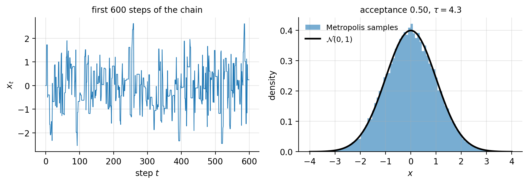
Figure 2.5: Metropolis sampling of an unnormalised standard Gaussian, Eq. (2.64). Left: the first \(600\) states of the chain, showing the correlation between successive samples. Right: the sampled histogram against the exact density.
Machine learning connection
The Metropolis algorithm is the sampling engine behind several of the generative models later in this book. Training a restricted Boltzmann machine requires expectation values over the model distribution, which are estimated by Gibbs sampling – a variant in which the proposal is a conditional distribution and the acceptance probability is therefore always unity. Bayesian neural networks sample the posterior over weights by Hamiltonian Monte Carlo, a Metropolis method whose proposal follows the gradient of the log-density. And the denoising process of a diffusion model is a learned approximation to the reverse of a stochastic chain of exactly this type. In all three cases the acceptance criterion (2.64) is doing the same work: it lets us sample from a distribution we can score but cannot normalise.
2.15. Summary and the programs#
The chapter has moved from probability to practice. The first part supplied the language: a stochastic variable is a domain together with a distribution, expectation values summarise that distribution through its moments, covariance measures linear dependence between variables, and the central limit theorem explains why averages become Gaussian and why their uncertainty falls as \(1/\sqrt{n}\).
The second part turned to what we actually compute. Every quantity extracted from a finite sample is an estimator, hence a random variable, and it is characterised by a bias and a variance which combine into Eq. (2.27). Two warnings were issued there and both are easy to forget: the \(1/\sqrt{n}\) law assumes independence, and when the data are correlated the effective sample size is \(n/\tau\) with \(\tau\) the autocorrelation time of Eq. (2.36); and an unbiased estimator is not automatically preferable to a biased one, since Eq. (2.27) counts variance equally. Applied to the least-squares estimator, the same machinery gave \(\var(\hat{\bm{\theta}})=\sigma^{2}(\bm{X}^{T}\bm{X})^{-1}\), tying the statistical uncertainty of a fit directly to the conditioning of the design matrix discussed in Chapter 1.
The third part concerned models rather than numbers. The bias-variance decomposition (2.52) explains the characteristic shape of the test error as a function of model complexity, and identifies the irreducible noise floor beneath it. The bootstrap manufactures the ensemble of training sets that the decomposition presupposes but that we never possess, and cross-validation organises the train-test split so that every observation is used for both purposes without ever being used for both at once. A single methodological thread runs through all of it: anything learned from the data must be learned from the training data only.
The fourth part dealt with producing randomness rather than analysing it. Pseudo-random generators supply uniform deviates, from which other distributions follow by inverse transform sampling, and when neither the normalisation nor the inverse cumulative distribution is available, the Metropolis algorithm samples using ratios alone.
The complete programs are collected in doc/BookML/BookPrograms:
distributions.py– the distributions of Section Distributions we shall need, with the plots reproduced here, and a numerical demonstration of the central limit theorem for several non-Gaussian starting distributions.estimators.py– sample moments, Bessel’s correction, the autocorrelation function and the correlation time of Eq. (2.36), applied both to independent data and to a correlated Markov chain.resampling.py– the jackknife and the bootstrap, the bias-variance decomposition as a function of polynomial degree, and \(k\)-fold cross-validation for the selection of a Ridge penalty.sampling.py– linear congruential and modern generators, inverse transform and Box-Muller sampling, and the Metropolis algorithm with an autocorrelation analysis of its output.
Each file runs as a script and reproduces the numbers quoted in this chapter. An executable version of the same material is available as a Jupyter notebook in the accompanying Jupyter-book.
2.16. Exercises#
2.16.1. Warm-up exercises#
Moments of familiar distributions. (a) Show that the uniform distribution (2.6) on \([a,b]\) has mean \((a+b)/2\) and variance \((b-a)^{2}/12\). (b) Show that the exponential distribution (2.10) has mean \(1/\alpha\) and variance \(1/\alpha^{2}\). (c) Verify Eq. (2.16), \(\var(X)=\mean{x^2}-\mean{x}^2\), for both.
Linearity and its limits. Prove Eq. (2.17), and then show that for two variables
\[ \var(X+Y) = \var(X)+\var(Y)+2\cov(X,Y). \]Under what condition do variances simply add? Explain why this is the identity behind Eq. (2.24).
Covariance without dependence, dependence without covariance. (a) Let \(X\) be uniform on \([-1,1]\) and \(Y=X^{2}\). Compute \(\cov(X,Y)\) and comment. (b) Construct two variables that are uncorrelated but not independent, other than this example. (c) Explain what this implies for a feature-selection procedure based on the correlation matrix alone.
The central limit theorem numerically. Draw \(m\) values from (a) a uniform distribution, (b) an exponential distribution, and (c) a Cauchy distribution \(p(x)=1/[\pi(1+x^{2})]\), and histogram the average over many repetitions for \(m=1,2,10,100\). Two of the three converge to a Gaussian with width \(\sigma/\sqrt{m}\). Which does not, and why does the theorem not apply?
Bessel’s correction. Prove Eq. (2.28). Then verify it numerically by drawing many samples of size \(n=5\) from a known distribution and comparing the average of the two estimators with the true variance.
Bias and variance of an estimator. Consider estimating the variance of a Gaussian by \(\hat{\sigma}^2_c = c\sum_k(x_k-\bar{x})^2\) for a constant \(c\). (a) Find the \(c\) that makes the estimator unbiased. (b) Find the \(c\) that minimises the mean squared error (2.27). (c) Are they the same? Comment on what this says about the value of unbiasedness.
Autocorrelation (numerical). Generate a correlated sequence by the autoregressive rule \(x_{t+1}=\phi x_t+\eta_t\) with \(\eta_t\) standard normal and \(\phi=0.9\). (a) Estimate the mean and its naive standard error (2.24). (b) Compute the autocorrelation function (2.35) and the correlation time \(\tau\). (c) By how much was the naive error underestimated? Compare with the prediction \(\tau=(1+\phi)/(1-\phi)\).
Variance of the least-squares estimator (numerical). Generate data from Eq. (2.37) with known \(\bm{\theta}\) and \(\sigma\). (a) Fit \(\hat{\bm{\theta}}\) many times with fresh noise and compute the empirical covariance of the estimates. (b) Compare with the prediction \(\sigma^{2}(\bm{X}^{T}\bm{X})^{-1}\) of Eq. (2.47). (c) Repeat with two nearly collinear columns in \(\bm{X}\) and relate the result to the singular values, using Eq. (1.122).
Bootstrap of a statistic without a formula. For a sample from a skewed distribution of your choice, use the bootstrap to estimate the standard error of (a) the mean, (b) the median, and (c) the ratio of the mean to the standard deviation. For which of the three could you have obtained the answer analytically?
Cross-validation and leakage (numerical). Take a data set with \(n=100\) observations and \(p=5000\) pure-noise features, entirely unrelated to the target. (a) Select the \(100\) features most correlated with the target using all the data, then cross-validate a model built on them. Report the estimated error. (b) Now perform the same selection inside each cross-validation fold. Report the estimated error again. (c) Explain the discrepancy in terms of the notebox of Section Cross-validation.
2.16.2. Exercise session: from probability to resampling#
Exercise 1: expectation values and the covariance matrix. Let \(\bm{X}=(X_0,\dots,X_{p-1})^{T}\) be a vector of stochastic variables with mean \(\bm{\mu}\) and covariance matrix \(\bm{\Sigma}\), and let \(\bm{A}\) be a constant \(q\times p\) matrix.
Exercise 2: the bias-variance decomposition.
Exercise 3: resampling and sampling.